Freelancing In Paradise

I took a career break while I was still living in the tropics and had the chance to do some freelance work in between SCUBA dives. One of my first gigs was to help a client to evaluate their sales target setting process. Their team was split into two groups and some rumours were circulating that one group had their targets set too easy. I was able to recommend some improvements based on some very simple statistical tests.

With the client’s permission, I’ve posted a brief write-up. This is a great demonstration of how easy it is to run Bayesian equivalents of standard statistical tests, using the BayesianFirstAid package by Rasmus Bååth.

Statistical Analysis of Sales Data #

Introduction #

The client’s sales department is organised into groups A and B. Members of Group B are set much lower quotas (sales targets) on average, reflecting an added difficulty to sell to group B customers.

Business Problem #

Is there any difference performance between the two groups? What (if any) anomalies are present? Make recommendations based on the findings.

Executive Summary #

Members of Group B are much more sensitive to quota size, with diminishing chances of meeting their quota as quota increased over a very small range. This appears to align with the additional challenge of selling to this customer segment. There is some evidence of a disparity between the two groups, with Group B members more likely to struggle to quotas as quotas increase. The same is not true of Group A and their chances of meeting quota.

Methodology #

I reviewed the descriptive statistics before analysing the groups using Bayesian statistical tests. Bayesian methods are preferred for this analysis because the data is a complete census (the entire sales department). The interpretation is more intuitive and I do not intend to make inferences about a larger population. Furthermore, checking assumptions and diagnostics for packaged Bayesian models is much less time consuming.

Descriptive #

The following listing shows the top 6 rows of the data file to show what a simple data set I was working with. The standard descriptive summaries are shown in Appendix A so I can jump directly to the more interesting parts of the investigation.

1
2
3
4
5
6
7
8
9

## # A tibble: 6 × 5
##   Group Attainment KSales KQuota MetTarget
##   <fct>      <dbl>  <dbl>  <dbl> <lgl>    
## 1 A          104.    33.7   32.4 TRUE     
## 2 A           92.6   25.0   26.9 FALSE    
## 3 A          109.    29.9   27.4 TRUE     
## 4 A          107.    24.2   22.6 TRUE     
## 5 A           92.9   23.2   25.0 FALSE    
## 6 A           98.2   24.7   25.1 FALSE

Initial Exploration and Impressions #

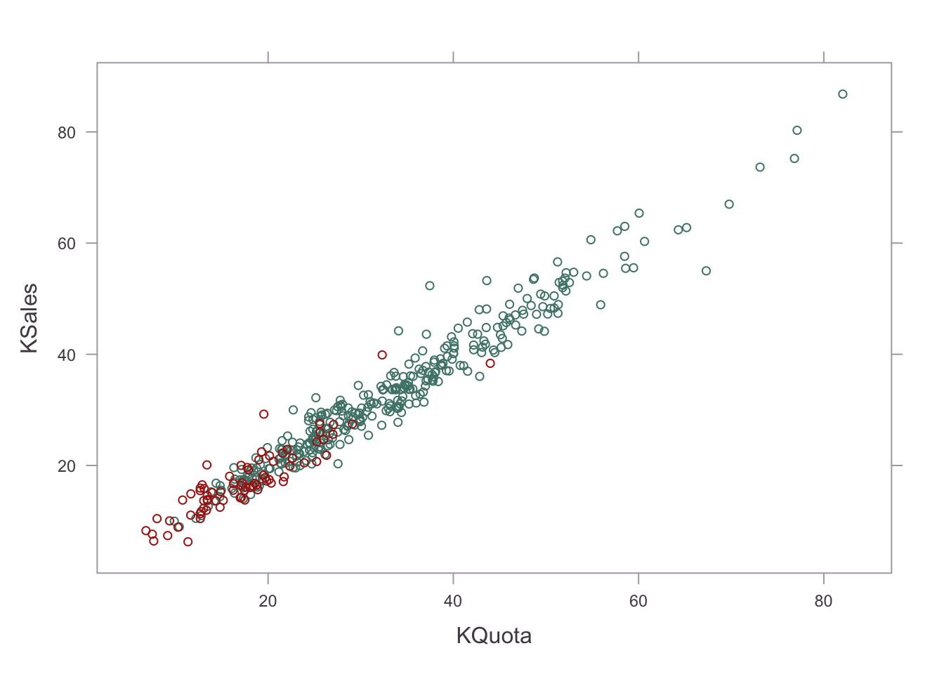
The obvious place to start the investigation is with a correlation analysis between quota set and sales achieved. I also visualise the relationship and colour according to group membership.

1

## Quota to Sales Correlation

1

## [1] 0.9776268

As expected, given the brief, Group B have lower mean quota and sales than Group A. There appears to be a very strong correlation between quota and sales. I asked the client to consider what this correlation implies. Does the person setting the quota (targets) at the start of the sales year have an uncanny grasp of the annual sales process? Are sales team members working up to the quotas but taking their foot off the gas when they know they’ve qualified for a bonus? If so, could a stretch target change the outcomes? These are causal questions that I could not possibly answer with this simple data set but it led to some interesting follow up discussions.

Differences in Performance Within Groups #

I considered the two groups separately, given the known difference between groups already described.

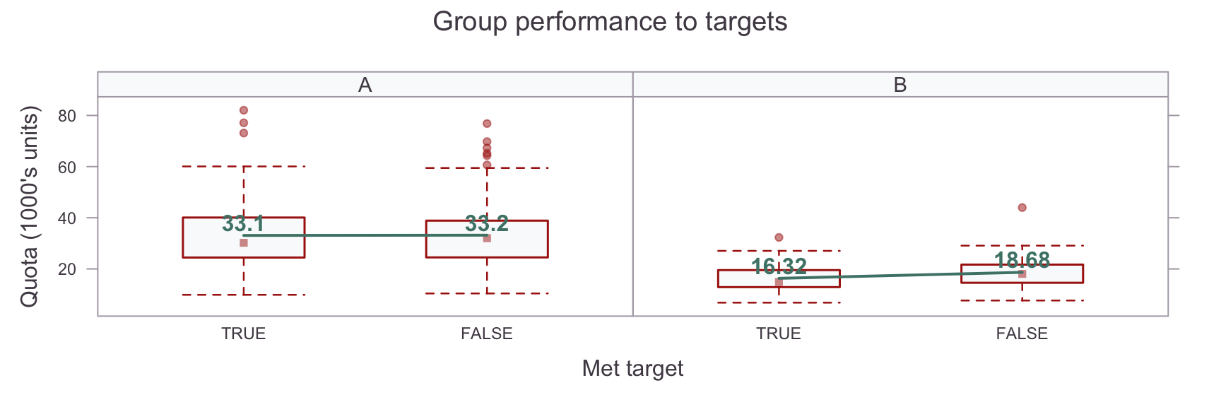
For those who made their targets compared to those who didn’t, it was useful to know how much their quotas were influential. A boxplot helps to visualise this for the two groups:

In Group A, there is no real difference in the mean Quotas ($\approx$ 0.1K sales quota units) between those who met their target and those who didn’t. For Group B, this difference is notably \(\approx\) -2.36K sales quota units i.e. somewhat lower among those who met their target than those who did not.

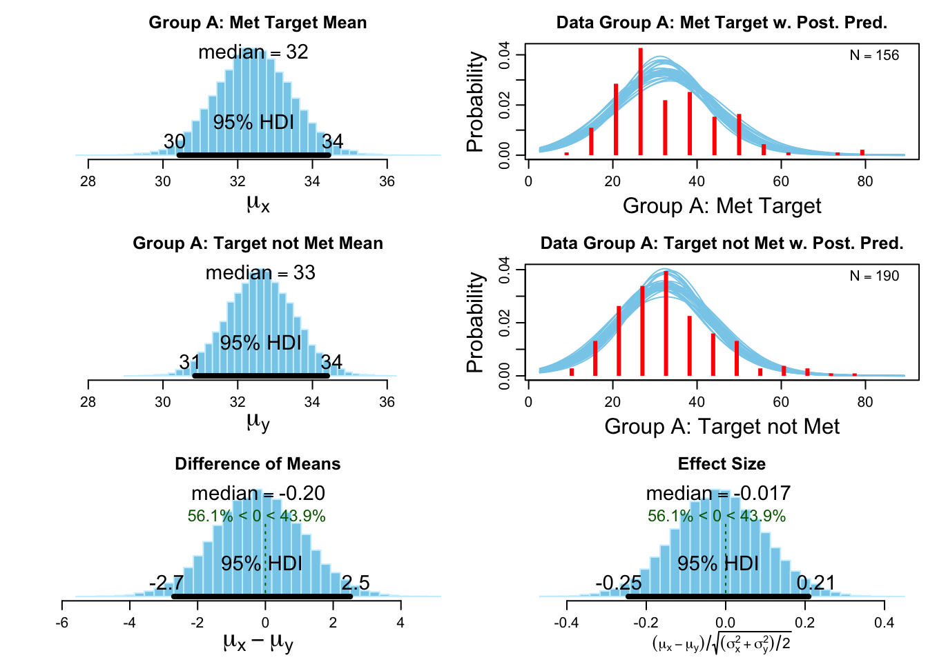
However, with such a large range of quotas (6.81, 32.32), is this difference important? A Bayesian t-test can help to answer this question. For comparison, I show the test results for both groups.

Bayesian t-test Group A #

The bottom two charts show the posterior (distribution) of the mean difference (Group A: Met Target vs Group A: Target not Met). I can see the posterior is centred very close to zero difference.

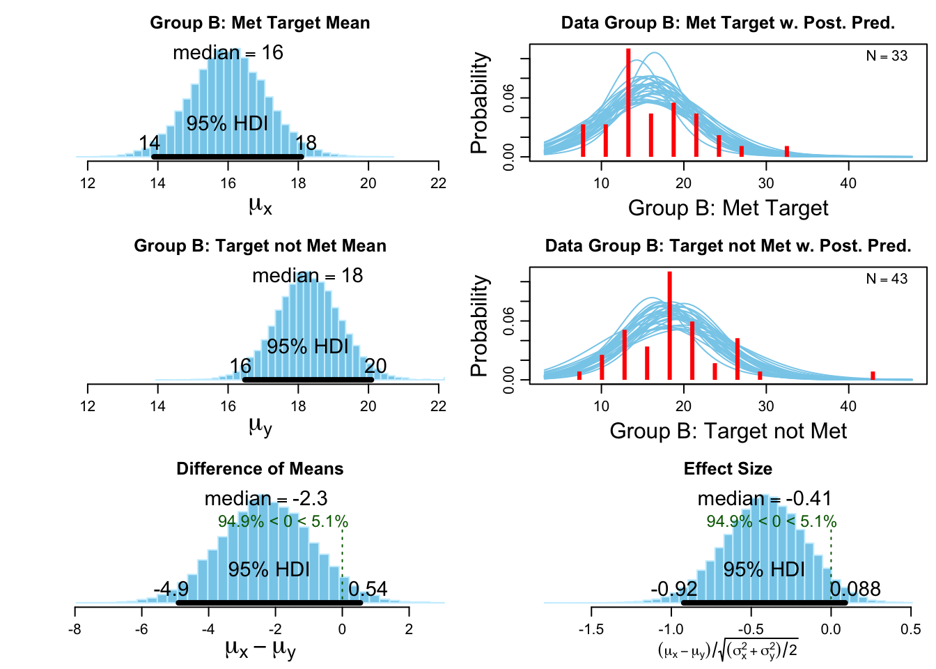
Bayesian t-test Group B #

The bottom two charts show the posterior distribution of the mean difference (Group B: Met Target vs Group B: Target not Met). I can see the posterior is centred at -2.27 which aligns with the above box plot. The effect size (relative to the variance) is considered medium at -0.41. Zero is inside the credible interval, but there is a \(\approx 95\%\) that the Met Target sub group have a lower median target than the Target not Met sub group.

Remarks #

The obvious difference between groups is expected, as per the client brief (different customer segments), so the groups were considered separately here. A Bayesian t-test confirms the visual assessment that there is no significant difference in the median quotas set for the sub-groups in Group A (those who met their target vs those who missed it). One the other hand, I found evidence to suggest that this is not the case for Group B. Those who met their targets (taken as a group) may have had slightly more achievable targets than those who did not. Note that the evidence is borderline credible.

A standard t-test (not shown) produced a very similar result but the difference in Group B would be reported as non-significant based on the p-values (p = 0.056). Again, I might consider this a borderline result but the Bayesian interpretation is more intuitive.

A visual analysis of the MCMC diagnostics (not shown) revealed no problems with the test convergence.

Conclusion #

In light of this finding I suggested a review of the quota setting for group B, in order to ensure fairness across the team.

Appendix A: Descriptive Statistics #

Here are the standard summaries for the whole sample, and separately by group.

1

## Both Groups

1
2
3
4
5
6
7

##  Group     Attainment         KSales           KQuota       MetTarget      
##  A:346   Min.   : 55.35   Min.   : 6.282   Min.   : 6.813   Mode :logical  
##  B: 76   1st Qu.: 93.25   1st Qu.:20.279   1st Qu.:20.714   FALSE:233      
##          Median : 98.68   Median :28.271   Median :27.791   TRUE :189      
##          Mean   : 99.37   Mean   :30.140   Mean   :30.363                  
##          3rd Qu.:104.00   3rd Qu.:37.284   3rd Qu.:37.786                  
##          Max.   :150.12   Max.   :86.803   Max.   :82.044

1

## Group A only

1
2
3
4
5
6
7

##  Group     Attainment         KSales           KQuota       MetTarget      
##  A:346   Min.   : 73.73   Min.   : 8.969   Min.   : 9.873   Mode :logical  
##  B:  0   1st Qu.: 93.88   1st Qu.:23.605   1st Qu.:24.513   FALSE:190      
##          Median : 99.11   Median :30.601   Median :31.171   TRUE :156      
##          Mean   : 99.37   Mean   :32.949   Mean   :33.154                  
##          3rd Qu.:103.75   3rd Qu.:40.309   3rd Qu.:39.982                  
##          Max.   :139.73   Max.   :86.803   Max.   :82.044

1

## Group B only

1
2
3
4
5
6
7

##  Group    Attainment         KSales           KQuota       MetTarget      
##  A: 0   Min.   : 55.35   Min.   : 6.282   Min.   : 6.813   Mode :logical  
##  B:76   1st Qu.: 87.72   1st Qu.:13.770   1st Qu.:13.089   FALSE:43       
##         Median : 95.00   Median :16.462   Median :17.322   TRUE :33       
##         Mean   : 99.33   Mean   :17.353   Mean   :17.656                  
##         3rd Qu.:107.80   3rd Qu.:20.534   3rd Qu.:20.392                  
##         Max.   :150.12   Max.   :39.890   Max.   :43.988

Appendix B: Code #

 1
 2
 3
 4
 5
 6
 7
 8
 9
10
11
12
13
14
15
16
17
18
19

library(readr)
library(dplyr)
library(lattice)
library(vcd)
library(BayesianFirstAid)
source("TC_Theme.R")
link <- "TC_SalesQuota.csv"
raw.data <- read_csv(link) %>%
  mutate(Group = as.factor(Group)
            , KSales = Sales/1000
            , KQuota = Quota/1000
            , Sales = as.integer(Sales)
            , Quota = as.integer(Quota)
            , MetTarget = Attainment >= 100)

get.col <- function(colnm, grp) {
  as.matrix(raw.data %>% filter(Group == grp) %>% dplyr::select(colnm))
}
set.seed(12321)

1
2
3
4
5
6

cat("Both Groups")
summary(k.data)
cat("Group A only")
summary(k.data %>% filter(Group == "A"))
cat("Group B only")
summary(k.data %>%  filter(Group == "B"))

 1
 2
 3
 4
 5
 6
 7
 8
 9
10
11
12
13
14
15
16
17
18
19
20
21
22
23
24
25
26

mns <- round(tapply(raw.data$KQuota, list(raw.data$Group, raw.data$MetTarget), mean),2)
mns <- mns[, c("TRUE", "FALSE")]
bwplot(KQuota ~ factor(MetTarget, levels = c(TRUE, FALSE)) | Group
       , data = raw.data
       , scales = list(format = list(digits = 10))
       , par.settings = MyLatticeTheme
       , strip = MyLatticeStrip
       , xlab = "Met target"
       , ylab = "Quota (1000's units)"
       , main = "Group performance to targets"
       , panel = function(x, y, ...) {
         panel.bwplot(x, y, ...)
         panel.average(x, y
                       , lwd = 2
                       , lty = 1
                       , col = myPalDark[1]
                       , ...)
         panel.text(1:2
                    , mns[which.packet(),] + 5
                    , mns[which.packet(),]
                    , col = myPalDark[1]
                    , cex = 1.1
                    , fontface = "bold"
                    , ...)
       }
)

1
2
3
4
5
6
7
8

tta <- bayes.t.test(get.col("KQuota","A")[get.col("MetTarget", "A")]
            , get.col("KQuota","A")[!get.col("MetTarget", "A")]
            , var.equal = TRUE)

tta$x_name <- "Group A: Met Target"
tta$y_name <- "Group A: Target not Met"

plot(tta)

1
2
3
4
5
6
7
8

ttb <- bayes.t.test(get.col("KQuota","B")[get.col("MetTarget", "B")]
            , get.col("KQuota","B")[!get.col("MetTarget", "B")]
            , var.equal = TRUE)

ttb$x_name <- "Group B: Met Target"
ttb$y_name <- "Group B: Target not Met"

plot(ttb)