To A/B or not to A/B
Last Updated:
Table of Contents
Introduction #
This is the story of a project that began as a straightforward A/B test but quickly revealed more than expected—offering fresh insights and expanding the scope of analysis.
It’s been a while since I worked as an independent data and analytics consultant. I went freelance after many years in data systems, BI, and MIS at a large multinational education company. During that time, I led projects using applied statistics, data mining, and algorithmic forecasting—and discovered a real passion for data science. But the chance to deepen those skills long-term wasn’t there, so I made the leap into freelancing, motivated by clarity about my goals and a desire for more hands-on, impactful work.
One of my first projects was with a startup language app—now a common genre, but at the time still rapidly evolving. These apps rely on gamified exercises, engaging features, and clever design to drive user retention and learning outcomes. Back then, much of that had to be figured out from scratch.
My client, still in the early stages, was looking to boost user growth with tactical feature launches tied to measurable impact. I was brought in to run a time-limited experiment: would a prototype for more interactive exercises lead to better word retention for new vocabulary? The results would inform whether to launch or revisit the design.
Disclaimer #
I’m grateful to that client for agreeing to partially lift our NDA so I could share this work. Enough time has passed—and the tech has evolved enough—that the study no longer holds commercial value. The company remains anonymous, and no personal or sensitive data is included here. The original dataset is not publicly available.
On the Product and Business Goals #
At the time of the project, the product used push notifications to prompt users to complete regular word retention exercises. These took the form of Flashcards, displaying a word in either the target or home (usually native) language. Users could tap buttons to flip the card, confirm memorisation, or skip. This was before gesture-based navigation was common on Android, so buttons were still the primary interface.
The new feature was more interactive—closer to a game. Users saw a sentence in the target language with a blank and had to choose the correct word to fill it from a set of options. The idea was that selecting the right word in context shows deeper understanding. Unlike Flashcards, which rely on self-reported memorisation, this approach generates more objective data on user progress. As a result, it could improve the accuracy of learning personalisation over time.
Strategically, the client was keen on Fill-in-the-Blank exercises for their potential to yield richer formative data. But they came with a trade-off: they were more cognitively demanding and time-consuming, raising concerns about lower engagement and increased churn.
Problem Definition #
The experiment compared two types of exercises—a simple two-level factor:
- Flashcards (control group)
- Fill-in-the-Blank (test group)
The primary goal was to assess whether these exercises led to different word retention scores, measured through separate weekly in-app vocabulary quizzes. We also aimed to evaluate differences in user engagement and churn between the two groups.
Experimental Hypotheses #
Word Retention #
\(H_0\)There is no difference in word retention score that depends on the type of exercise - Flashcards vs. Fill-Blanks\(H_a\)There is a difference in word retention score that depends on the type of exercise - Flashcards vs. Fill-Blanks
Here, the hoped-for outcome is that \(H_0\) can be rejected.
Churn Rate #
\(H_0\)There is no difference in churn rate that depends on the type of exercise - Flashcards vs. Fill-Blanks\(H_a\)There is a difference in churn rate that depends on the type of exercise - Flashcards vs. Fill-Blanks
Here, the hoped-for outcome is that \(H_0\) cannot be rejected.
Confounding Factors #
While designing the experiment, we quickly identified several potential confounding factors:
-
Engagement bias: If users engage differently with the two exercise types, retention scores could be affected independently of the exercise’s actual learning value. Since participation couldn’t be enforced, lower engagement with Fill-in-the-Blanks might reflect usability issues rather than learning efficacy. Some mitigation—like improving the prototype’s appeal—was considered.
-
Time-based effects: Learning outcomes or churn impacts might take longer than a single week to materialize. A short-term test could miss these delayed effects.
-
Survivor bias: If churn rates differ between groups, we risk measuring outcomes only among the more persistent users. This could inflate performance metrics for the group with higher dropout rates.
Hypothetical User Model #
To clarify some of our thinking about confounding factors, together with the client we developed a more sophisticated hypothesis about the existence of latent and causal factors. This is represented in the diagram below.
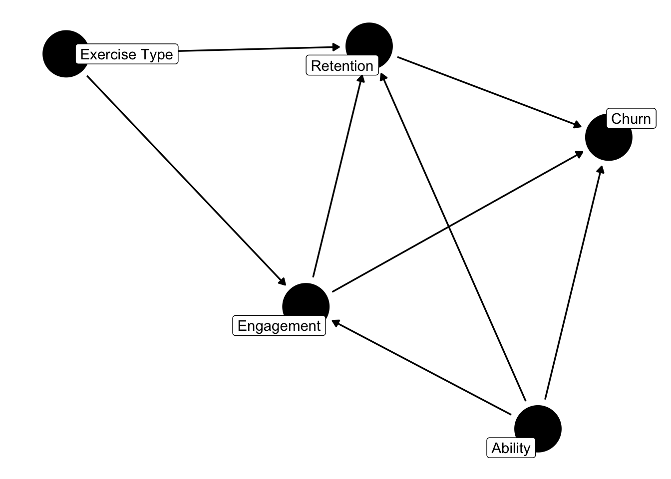
We developed a hypothetical model of the user, assuming each had a latent, unobserved ability. While not directly measurable, this ability could influence how engaged users were, how easily they retained vocabulary, and their likelihood of churn. Users with lower latent ability would likely face more difficulty and need greater resilience to stick with language learning.
As a startup focused on rapid growth, the client was especially wary of anything that might increase churn. Even a short-term experiment carrying that risk was a concern. Minimising this risk—while still running a meaningful test—was a key part of my role, and heavily influenced both the experimental design and the analytical approach.
Experimental Design #
Given the confounding factors, a simple A/B test followed by a t-test at the end of each week wouldn’t suffice. That approach would overlook two key sources of bias:
- Indirect effects: Fill-in-the-Blank exercises could affect retention scores indirectly by altering engagement levels.
- Survivor bias: If lower-performing users churned at higher rates due to the added effort required, this would skew group averages.
To address this, I proposed a set of guiding principles to structure the experiment in a way that would let us assess these effects in a single pass:
- Random assignment: To control for latent ability and user preferences, users were randomly assigned to one exercise type.
- Consistent exposure: Each group remained on the same activity for the full duration to allow us to detect differences in engagement and churn over time.
- Limited duration: The experiment would run for four weeks to reduce the risk of users churning simply due to prolonged exposure to a potentially less enjoyable feature.
- Minimised exposure: We limited the number of users in the study to further reduce potential churn impact during this critical growth phase.
Sample Size Calculation #
The client agreed on a minimum detectable effect (MDE) of 2 additional words retained per week. This would translate to a gain of roughly 108 words annually—modest, but meaningful—on top of a baseline of about 20 words per week (or 1,040 per year). Naturally, they were hoping for more, but this was set as the threshold for meaningful improvement.
Historical data showed a standard deviation of 4.87 in weekly word retention scores, which provided a useful input for estimating sample size. However, we also had to factor in churn: around 25% of users didn’t engage with the app for at least one week during any four-week period. To ensure we had sufficient completions to maintain 80% statistical power, I adjusted for this dropout risk.
I used the short-hand formula -
$$N \approx \left(\frac{8\sigma}{\Delta}\right)^2$$
to estimate the total sample size, which gave me
$$ \left\lceil \left(\frac{8 \times 4.87}{2}\right)^2 \right\rceil = 380 $$ This gave us a quick, practical estimate to review feasibility with the client.
Later, I validated the result using power.t.test in R and adjusted for churn by inflating the required sample size, using a conservative adjustment based on the churn rate plus two standard deviations (via \(\sigma^2 = p(1-p)\)).
|
|
The final result was:
|
|
I don’t know why but it was weirdly satisfying that such a nice round number popped out by pure chance.
Participation in the Trial and Managing Churn #
Although the sample size was padded to account for churn, we still needed to monitor it closely during the trial. Crucially, we couldn’t exclude users who dropped out—doing so would introduce survivor bias. Users had to be entered into the trial at random, and their outcomes included, regardless of whether they completed the full period.
From a larger pool of about 10,000 users, we randomly selected 400 users using R’s random number generator and assigned them to one of two groups. For exactly four weeks, each participant received two push notifications per week, prompting them to complete a vocabulary retention exercise based on words previously encountered in the app.
Each user was assigned a set of metrics:
- Per-user:
- exercise_type (treatment factor): “Fill-Blanks” or “Flashcards” — the only exercise type they saw during the trial.
- churn_week (int): The first week in which the user didn’t use the app at all; if they were active all four weeks, this was set to 5.
- churn (factor): “churned” if churn_week < 5; otherwise, “completed trial”.
- Per-user, per-week:
- engagement (factor): “High” if the user completed at least one exercise that week, “Low” otherwise. If a user churned, engagement was set to “Low” for that week and all subsequent ones.
- retention (int): The number of words correctly retained in the weekly quiz. If the user churned, this was set to NA for that and all future weeks.
Interlude #
In the meantime while I was agreeing these parameters with the client and his team, the developers were preparing the A/B test framework. They confirmed that once a user was allocated to a test group, they would only see one type of test for the four week duration and the requested data would be collected weekly. All other users would continue with business as usual.
There was nothing left to do but run the trial. I took a short SCUBA diving break and then worked with another client for a couple of weeks.
Results Analysis Part 1 - Preliminaries #
Immediately after the test period completed, I collated the data for an initial review.
|
|
Here we can see that the grand mean engagement over all users, all weeks was 0.73438, while the mean word retention each week was 22.19317. The number of NAs in this result set looks high but there are duplicates. A user who churned in week 1 would present as 4 NAs. The actual number of churned users was counted separately but can also be determined by looking at the fourth week results only. This was found to be 90, which is 0.22 on a total N of 400 (two groups) and slightly below our pre-study expectation.
Summary Statistics by Treatment/Control and Weeks #
I tabulated all the weekly metrics that we had collected and summarised their means and standard deviations, as shown here.
|
|
Observed Four Week Churn Rates #
Aside from the retention and engagement means, we also took the opportunity to check the churn rate. In particular, the four week churn rate was of interest.
|
|
The rate for Fill-Blanks was in line with the prior expectations but the rate for Flashcards was a bit lower. Was this significant? I did a quick log odds ratio test to find out.
|
|
The large p-value indicated that that their was no evidence of a significant difference. I plotted the counts to double check.
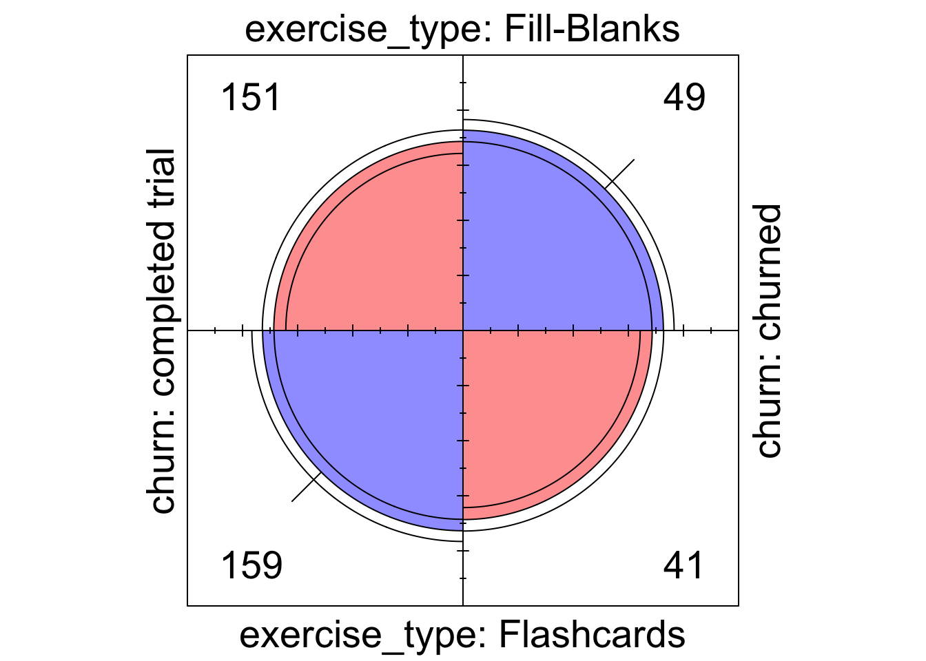
The non-finding was backed up by the fourfold plot, which showed overlapping confidence intervals of the quarters. The difference in churn rates was entirely within the margin of error. Nevertheless, I chose to reserve my final judgement until I had a chance to look more deeply at the other results.
Naive T-Test #
Sometimes, the only required analysis for an A/B test is a t-test to check for a statistical difference in means between groups, assuming everything has gone well with the experiment. We knew that wasn’t the case here but it’s always an informative measure.
I started by taking mean weekly retention score per user, so long as they didn’t churn in the first week of the study. This was calculated by summing up their individual weekly scores and dividing by the number of weeks that they remained unchurned.
|
|
Then I ran the Student’s t-test to get an initial intuition of whether the whole endeavor had yielded a statistically interesting result.
|
|
These results suggested a statistically significant difference in means of between 0.77512 and 1.95348 with a confidence of 0.95 among users who were given Fill-Blanks exercises over users who were given Flashcards exercises. I noted that the upper bound was below the minimum detectable effect of 2 that we had agreed before starting but it was too early to be disappointed. The possible presence of confounding factors required a deeper analysis.
Results Analysis Part 2 - Engagement #
One of my first priorities was to verify some of our initial assumptions. Did the level of engagement depend on the exercise itself? Also, over the weeks of the study, did the users show a growing or diminishing level of engagement? This information would shine a light on our hypothetical user model and reveal any important interactions.
Analysis of Variance #
The quickest way to check is with an ANOVA test.
|
|
According to this result, there is a statistically significant effect on engagement depending on the type of exercise, but there is no detectable difference each week.
Mosaic Visualisation and Significance Tests #
A visual analysis can help to better understand what is happening.
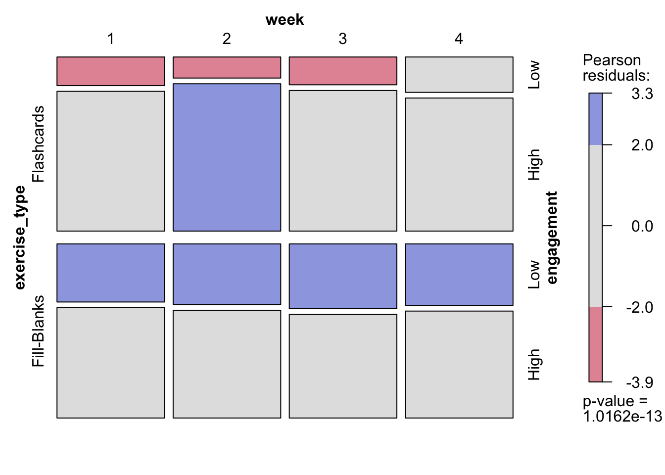
I’m a strong advocate for mosaic plots when working with count data like this. I’ve taught workshops on them because, while they can be unfamiliar at first, they’re incredibly revealing once you know how to read them.
The plot recursively divides a canvas by the specified categorical factors, with tile area proportional to counts at each intersection. If the factors are independent, the result is a neat grid. The more skewed or uneven the tiles, the stronger the interactions between variables. Tiles are shaded by Pearson residuals from a \(\chi^2\) test of independence — essentially embedding a statistical test into the visualization. Blue tiles (positive residuals) mark over-represented combinations; red tiles (negative residuals), under-represented ones.
What did this analysis reveal about user engagement?
As expected, the distribution across exercise type (Flashcards vs. Fill-Blanks) and week was even, since users were assigned randomly and engagement was recorded weekly regardless of churn. The striking difference appeared in engagement levels: Low engagement was clearly over-represented among Fill-Blanks users.
The implication was straightforward — users were more likely to complete Flashcard exercises. This aligned with expectations: Flashcards are quicker and cognitively lighter — users can simply tap through and self-confirm memorisation. The pattern held consistently over time, suggesting the effect was inherent to the mechanics of the exercises rather than a temporary novelty or fatigue effect.
Causal Analysis #
The key question was this: How much did lower engagement with Fill-in-the-Blank exercises affect overall word retention?
The client and I had anticipated that these exercises might see lower engagement — or even higher churn — which would be counterproductive, especially if it masked what could otherwise be better learning outcomes. To understand this dynamic, I needed to go beyond basic group comparisons and look into causal pathways.
I was already somewhat familiar with structural equation modelling (SEM) from past work on student surveys, but this problem—where an independent variable (exercise type) may influence the response (retention) indirectly through a mediator (engagement)—called for a more targeted approach.
While researching, I came across the mediation package in R, which seemed tailor-made for this use case. To build confidence in the results, I ran two parallel analyses: one using the mediation package, and another using a more traditional SEM approach, allowing me to compare the outputs and validate the findings.
Mediation Analysis #
|
|
This model does not take into account the repeated measures occuring each week. Despite the earlier ANOVA test and mosaic plot confirming that this wasn’t a particular concern here, I wanted to be very cautious when interpreting the results numerically.
The summary above shows a significant result for Average Causal Mediation Effect (ACME) of -0.21886. Any significant result here is evidence to reject a null hypothesis of no indirect effect. The ACME has the opposite sign of the Average Direct Effect (ADE) at 1.51281, which suggests that the total effect is less than it otherwise would have been.
I checked alignment with my preliminary result (from the earlier t-test) and found that the total effect of 1.29395 is close to the mean difference between groups of -1.3643. So this causal analysis seems strongly to suggest that the mean difference would have been larger by 0.21886 or some quantity between the ACME confidence interval, shown in the summary above.
Structural Equation Model #
I have used SEM to model latent factors before but had not tried using them to model a mediation effect. Anyway, the approach is pretty much the same except that there aren’t any latent factors, only manifest items. I conducted the analysis in much the same way as I would usually do it.
|
|
Here we’re seeing very well aligned results to the mediation method, with a direct effect of exercise_type on retention of 1.51281 and an indirect effect of exercise_type on engagement of -0.18724.
It’s also possible to plot the SEM, which is why I wanted to run the analysis this way.
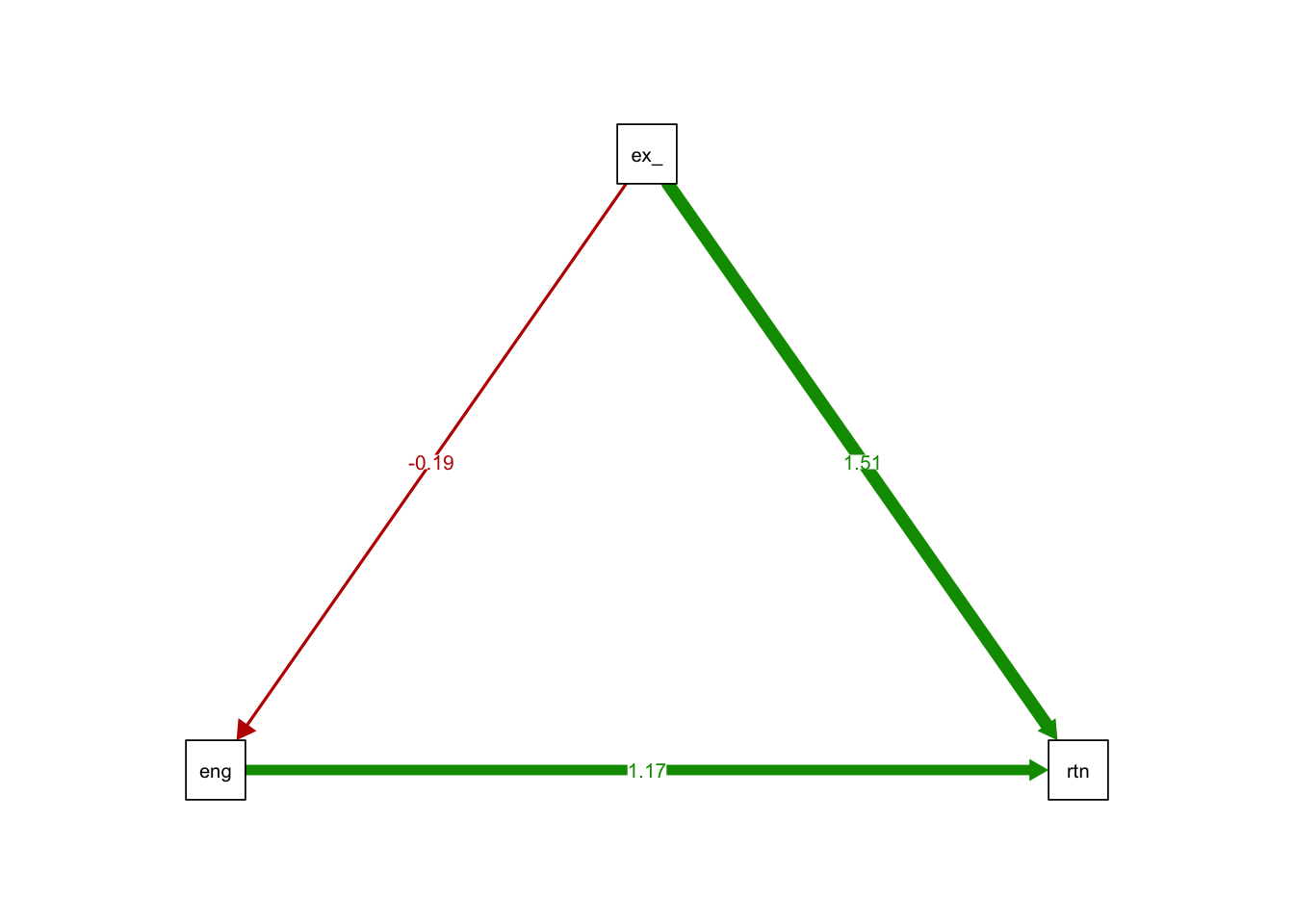
This was a very nice, simple visual for explaining to the client that Fill-Blanks has a downward effect on engagement, which must have a dampening effect on any increases in retention for users in the Fill-Blanks group.
Results Analysis Part 3 - Word Retention #
This stage of the analysis required the use of a linear mixed model (LMM) for one simple reason; given that we were tracking the users over the course of four weeks, with one overall retention measure per week, the experimental design is repeated samples, which violates the independence assumptions of an OLS linear model. I proceeded by working through a hierarchy of models, increasing the number interaction terms, to determine the best fitting model.
Linear Mixed Model Selection and Analysis #
As LMM are quite a bit more complex than linear models, there is a lot more to the summaries and consequently more console output. For brevity, I only post the best fitting model summary here, after the ANOVA test to determine the best fit.
|
|
Above you can see the model definitions. The notation shows that user_id has been set as a grouping variable with different intercepts but not different slopes. This means that the model’s intercept is modulated by each user’s random effect (their latent ability, in our user model).
Model mm2, with an interaction term between exercise_type and week is found to be a significantly better fit to the data than model one. The additional interaction term in model mm3 does nothing to improve on mm2. Therefore, mm2 was selected as the best fitting model. The model summary and diagnostics are shown next.
|
|
Note that there are 376 groups (user_id) discovered, which accounts for all users who didn’t churn in the first week. Then there are 1377 observations overall, which accounts for NAs for users who churned on any week after that, providing at least one but fewer than four observations to the study.
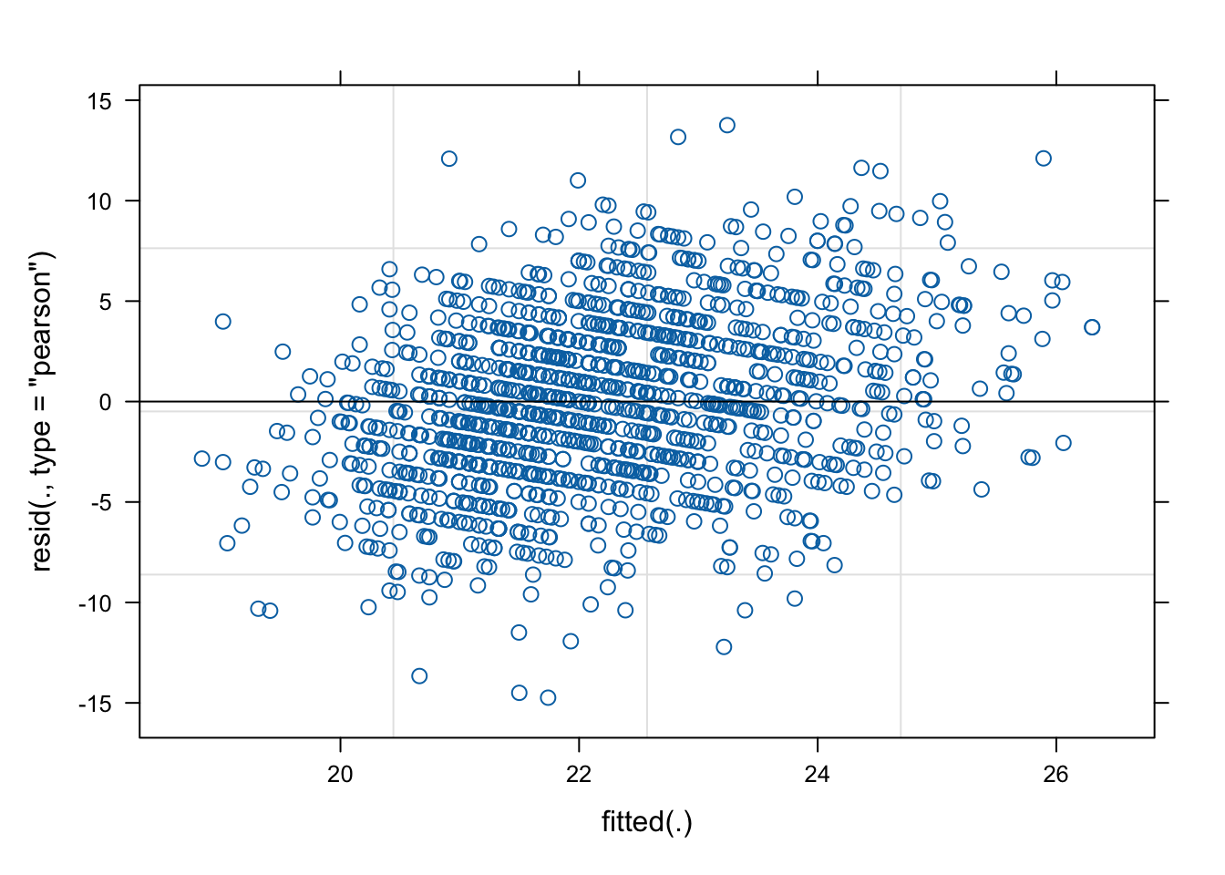
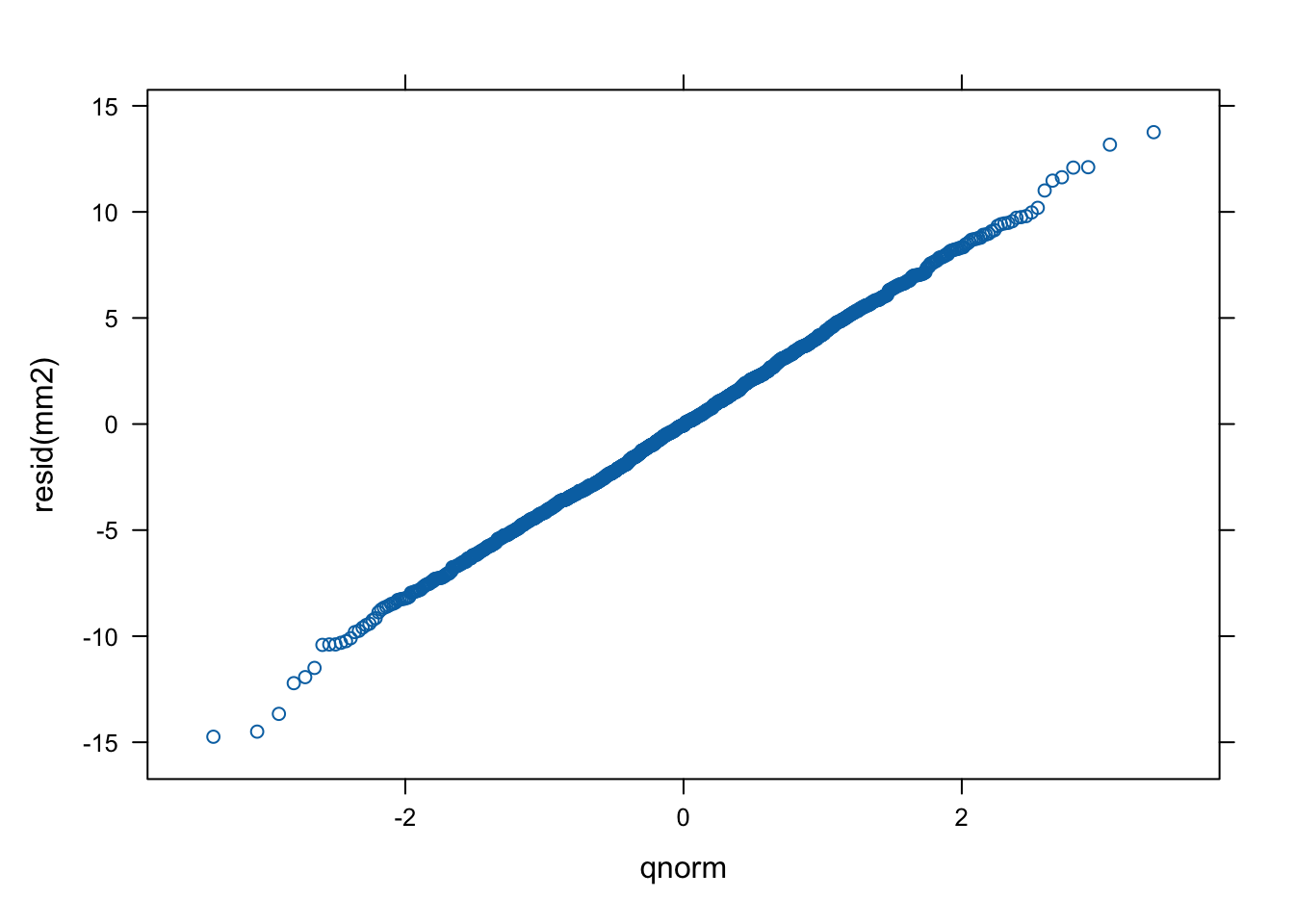
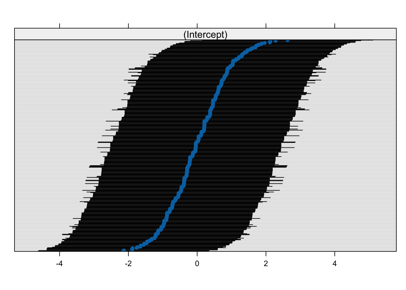
Model Diagnostics #
The model converged without any problems and the scaled residuals are centred on zero. This is also visible in the residual plots. The qqplot looked perfectly normal (no pun intended), and the random effects plot showed symmetry around zero, suggesting a normal distribution for the latent ability factor, as one would expect.
|
|
Sense-Making the Linear Predictor for Word Retention #
The model coefficients, as given in the summary, are significant for engagement, week, and the interaction between exercise_type * week but notably not for exercise_type main effect. This indicated to me that there is a significant difference between the two exercises but it does not become apparent until the later weeks of the study. I simplified the model accordingly by removing the non-significant main effect and used the ANOVA test to ensure that my simpler model was just as effective in explaining the variance in the retention scores.
|
|
The Simplified Model and Easy Explanations #
The parameter set of the simplified model was much easier to explain to the client.
|
|
The interpretation of these results is as follows:
- the baseline expectation is 20.41639 but has some variability, given individual users’ innate ability
- two standard deviations of this user variability on the baseline is plus or minus 1.96 * 1.55007 (possibly predictable in future from data collected from in app activities)
- if engagement is High, there is an additional 0.87234
- for each week up to four (so as not to extrapolate beyond the experimental conditions), there is an additional 0.73028 for Fill-Blanks exercises
- the 0.13931 per week for Flashcards exercises is within the margin of error and can be ignored
- as a result, there is a difference between the word retention scores for Fill-Blanks vs. Flashcards that accumulates over four weeks to 2.92112 (or more meaningfully, 3 additional words) compared to using only Flashcards
- additionally to keep in mind, the more time-and-effort consuming Fill-Blanks tasks is depressing the engagement level, which is counter-productive to the average retention scores for those same users
This plain English explanation made the most sense to my client and their team. I did not attempt to fully quantify the last point because it was the output of a separate modelling procedure. I did explain, however, that we should really be seeing a different engagement coefficient per exercise type but the LMM was not a suitable tool for discovering it because it does not discover relationships between independent variables. Rather, these relationships introduce bias.
A Mildly Shocking Oversight #
Going back to the experimental design parameters, I suddenly realised that our sample size was flawed. This difference in retention scores over four weeks is statistically significant to at least a 95% confidence level. The MDE was set at 2, which meant that I could be sure with 80% confidence that this difference was not in danger of being a false positive,
Unfortunately, I had made an error with the sample size calculation. The client had sought confirmation (with power 0.8) of their MDE of 2 words per week for a total of 8! This would have resulted in a drastically smaller sample size. All things considered, this issue was not a material cause for concern in the end because a much smaller sample could easily have been thrown off by an unusually high churn week, for example. Also, the numbers were still very small with respect to the total number of users. I can laugh about it now but I was quite embarrassed at the time.
Results Analysis Part 4 - Churn Rate #
I was still tasked with identifying whether the extra effort of completing a Fill-Blanks exercise would have an adverse effect on churn rate. So far, I had a bit of evidence from the four week churn rate for just the Fill-Blanks group staying in line with prior expectations. Also, even though the Flashcards control group did appear to be a little lower, there was the non-significant log odds ratio test, reducing any major concern. Nevertheless, I wanted to complete the analysis that I had planned and that data had been collected for.
I proceeded with a non-parametric survival analysis by using the per user data described above. This contains the churn week or 5 if they made it to the end of the study (as the majority did). A boolean churn event of TRUE for those who did churn, and a weekly average retention for the weeks they participated. Finally, there was also the exercise type, of course.
Between Groups Log-Rank Test #
It’s easy to compare survival distributions between groups using the log-rank test
|
|
The test shows that there is no significant difference between the two groups’ survival. However, this method does not control for retention, which is a concrete measure of the user’s learning progress. Our hypothetical user model, based on intuition and experience in the sector, suggested that it was a possibility that users who felt they were under-performing might be more likely to churn. So I went ahead and checked that as well.
Cox’s Proportional Hazards Model With A Continuous Variable #
I’ve discussed Proportional Hazard (PH) models in a lot more detail in this post so I will skip over the intricacies and just say that if we find a high value for hazard at any given moment, the survival rate is falling fast. Conversely, we might say that the churn rate is going up. It’s usual to report on the log hazard and check for values that a greater than zero with statistical significance.
For continuous independent variables, it is necessary to fit a smooth spline predictor in place of the raw data. The model reports on the linear part and non-linear part separately.
|
|
Notice here the number of observations used in the model is 376, just as we saw with the LMM. Given that there were 400 individuals to begin with, this means 24 individuals churned on week one and contributed no retention data. This made a full analysis impossible but I noticed that only the non-linear partition of the retention data returned a significant result.
The PH terms can be plotted, which sometimes helps with a non-intuitive analysis as we have here.
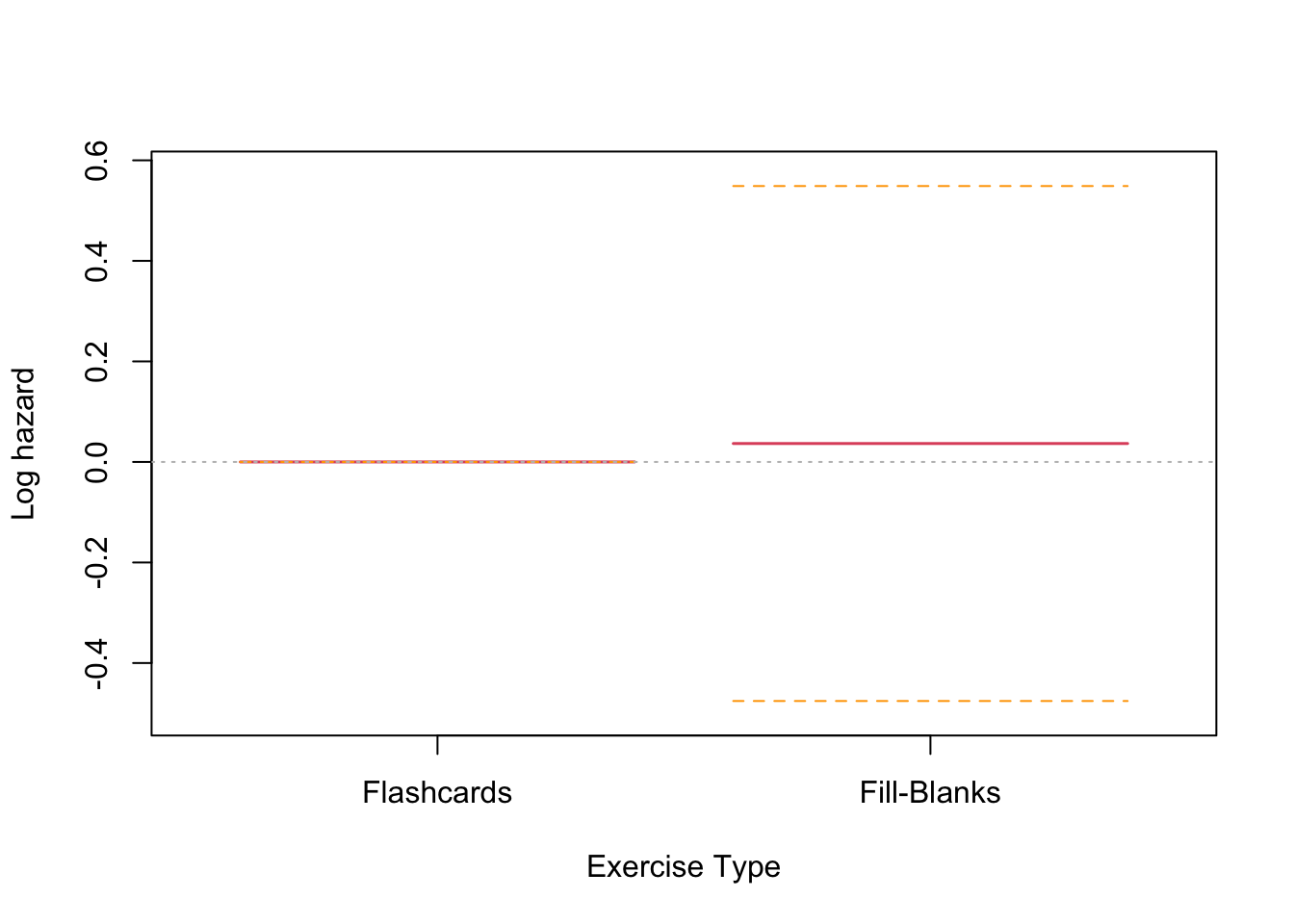
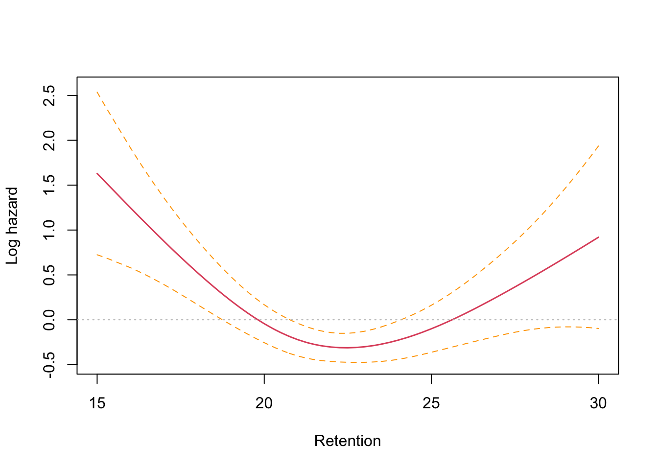
We see from these plots that the partial PH for the exercise types is close to zero, as the modeling suggests. The retention curve does appear to show a significant divergence from zero, certainly at the lower end. This aligned with the ideas we had in creating the user model at the beginning of the project - the mechanism being that users who are doing less well at memorising vocabulary are more likely to get frustrated stop returning to the app for many days at a time, or for good.
Survival Model of Churn #
As a final sense check, I created a survival model. Think of it as the reverse of churn. The greater the survival rate, the lower the churn rate in a direct \(p, 1 - p\) relationship. The survival plot provided me with the ideal way to communicate my churn rate analysis to the client because it is such an easy to understand visual.
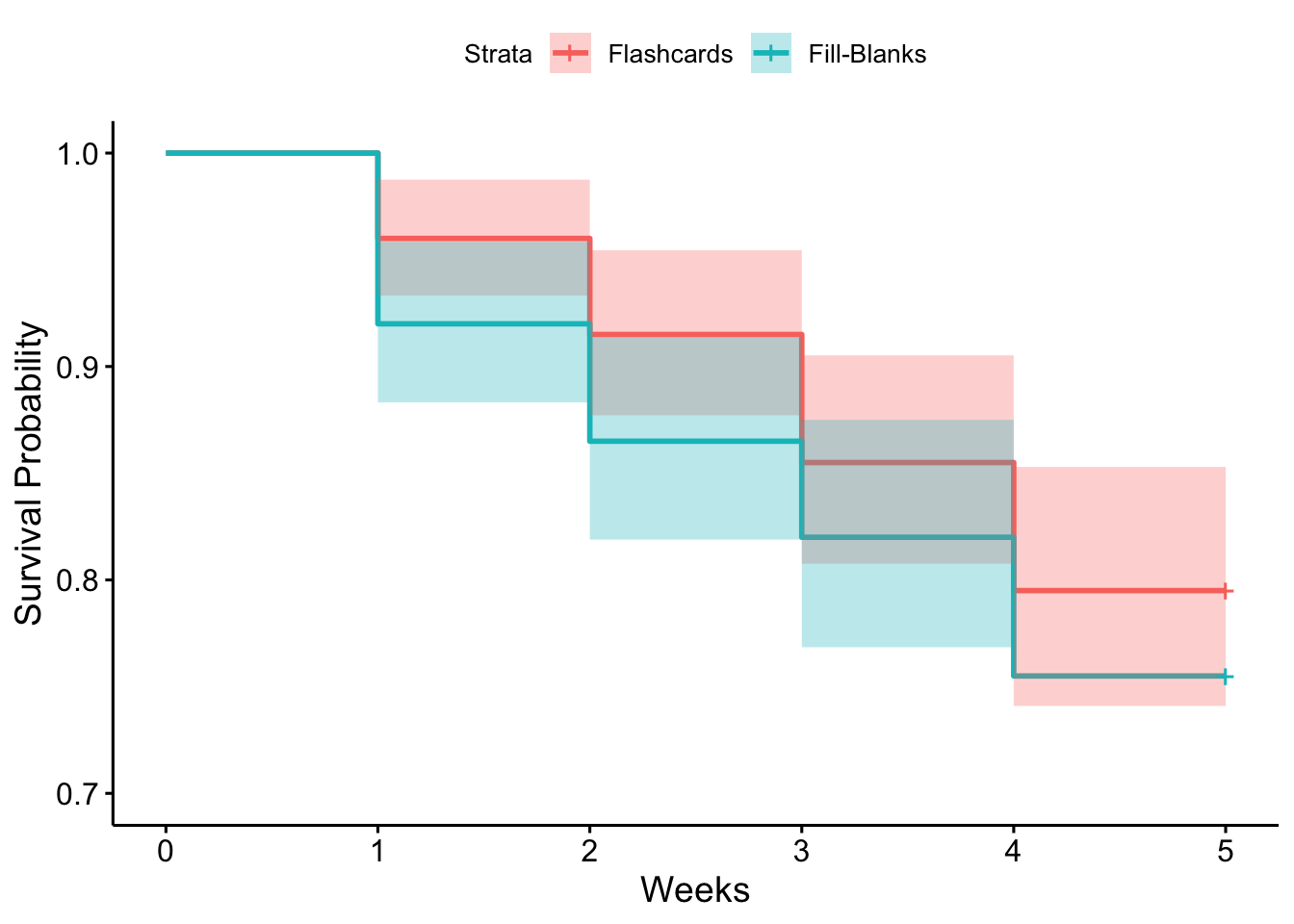
Certainly there is the appearance of a slightly lower survival rate for the Fill-Blanks group but it is very small and well within the margin of error. Happily, we could pretty much rule out the new Fill-Blanks exercise as a significant cause of increased churn risk.
Summary #
What began as a simple A/B test for a new vocabulary exercise evolved into a more complex analysis once we examined the client’s goals and the dynamics of the product. A basic t-test wouldn’t have captured the nuanced interactions at play.
By developing a user model with latent ability as a key concept, we identified several important confounding and mediating variables—particularly engagement and churn—that needed to be accounted for. This led to a multi-variate analysis approach, including a linear mixed model to handle repeated measures per user and individual-level variance.
To explore the causal pathway between exercise type, engagement, and retention, I used two methods: the mediation package and structural equation modelling (SEM). While I didn’t quantify the indirect effect precisely, both analyses helped clarify that engagement did mediate the impact of the exercise format on retention — albeit to a modest degree.
Key findings:
- The new Fill-Blanks exercises improved average word retention by approximately 3 words over four weeks.
- This improvement was lower than the client had hoped.
- The indirect negative effect of reduced engagement was present but relatively small in magnitude.
- Most importantly, we found no evidence of increased churn risk among users exposed only to Fill-Blanks exercises.
Conclusions #
This project was a powerful reminder that data science is about more than running models — it’s about framing the right questions and understanding the context in which data is generated.
The client’s openness to a deeper analysis allowed us to uncover insights that went beyond surface-level metrics. Although the headline result wasn’t transformative in terms of retention gains, the finding that Fill-Blanks exercises didn’t drive up churn gave the client confidence to move forward with the launch. The feature offered strategic advantages: better formative assessment data and continued product evolution to keep users engaged.
For me, this work reinforced a key lesson: deep domain understanding, clear causal thinking, and honest evaluation of trade-offs are what transform a data project from informative to actionable. It was a rewarding collaboration—and a great example of the kind of analytical thinking I always aim to bring to client work.
Appendix #
Here you can find the source code.
|
|