Optimize Like a Pro With LSD

Introduction #

Start-ups often need to move faster than traditional A/B testing best practices allow. Typically, A/B tests need a couple of weeks to gather enough data, sometimes more. When multiple improvements are ready to ship, waiting to test them one at a time can mean lost momentum or missed opportunities. Enter the Latin Square Design (LSD), a brilliant example of working smarter instead of harder. As a result of using LSD, your estimate of the treatment effect has significant sources of noise removed, which means:

• Fewer users required to detect a real effect with sufficient power.
• Random fluctuations in behavior across known sources of variance don’t affect your results.
• You reduce the risk of confounding effects muddying your conclusions.

In this post, I’ll walk through a recent scenario where the LSD turned out to be the perfect choice.

Overview of Latin Square Designs #

LSD is a statistical power tool that lets you test multiple treatments while controlling for two nuisance factors, all without blowing up your sample size or adding noise to your results. It cleanly separates the treatment effect from two known sources of variability. What’s striking is that thanks to the way it’s set up, LSD drastically reduces the number of test conditions you need to run while maintaining statistical power!

Instead of testing every possible combination (which would require $t\times r\times c$ runs for $t$ treatments and $c,r$ levels of each factor), the LSD only needs $t\times t$. That’s a major win-win.

How does it work? The secret lies in its structure. Each treatment is assigned in such a way that it appears exactly once in every row and column of a square layout — ensuring a balanced representation across both blocking factors. Here’s what that looks like for three factor levels:

The catch? Latin Square designs require the number of treatments to match the number of levels in each blocking factor to form the square. That symmetry requirement is what makes LSDs elegant — but also a bit rigid. If your real-world variables don’t fit neatly into this shape, more flexible alternatives like randomized block designs or factorial designs might be a better fit.

Just Enough Theory #

As with all my posts, I like to cover just ennough theory to allow readers to implement things for themselves. Fortunately, that’s not very much to grasp the basics of LSD.

Mathematically, the model looks like this:

$$Y_{\mathit{\text{ijk}}}=\mu +{\alpha }_i+{\beta }_j+{\tau }_k+{ϵ}_{\mathit{\text{ijk}}}$$ Where:

• $Y_{\mathit{\text{ijk}}}$ is the observed response (e.g., conversion)
• $\mu$ is the overall mean
• ${\alpha }_i$ is the row effect
• ${\beta }_j$ is the column effect
• ${\tau }_k$ is the treatment effect
• ${ϵ}_{\mathit{\text{ijk}}}$ is the random error

By explicitly controlling for two known sources of variation (the blocking factors) before estimating the treatment effect, the total (T) variance in the observed data is partitioned into several components: row (r), column (c), treatment (t), and residual error (e). These components are easily discovered by creating a standard ANOVA table and show up as the sum of squares (SS):

$${\text{SS}}_T={\text{SS}}_r+{\text{SS}}_c+{\text{SS}}_t+{\text{SS}}_e$$

You can also determine the relative efficiency (RE) of the design compared to a standard A/B test, one that would use a Complete Randomized Design (CRD) instead for the two blocking factors by the following formula:

$$\text{RE}=\frac{{\text{SS}}_e^{\text{CRD}}\times {\mathit{\text{df}}}^{\text{Blocked}}}{{\text{SS}}_e^{\text{Blocked}}\times {\mathit{\text{df}}}^{\text{CRD}}}$$

where ${\text{SS}}_e^{\text{CRD}}$ is estimated from the unpartitioned sums of squares:

$${\text{SS}}_e^{\text{CRD}}={\text{SS}}_r^{\text{Blocked}}+{\text{SS}}_c^{\text{Blocked}}+{\text{SS}}_e^{\text{Blocked}}$$

and the residual degrees of freedom (df) for the CRD is the df for the LSD plus the df for the factor components:

$${\mathit{\text{df}}}^{\text{CRD}}={\mathit{\text{df}}}_r^{\text{Blocked}}+{\mathit{\text{df}}}_c^{\text{Blocked}}+{\mathit{\text{df}}}_e^{\text{Blocked}}$$

When $\text{RE}>1.0$, the design is more efficient than the equivalent CRD (or standard A/B test). The greater the blocking effect (i.e., the larger the difference between the blocks), the more efficient the design becomes.

If you find RE is less than one, a common cause is that there is not much between block variability. The statistical effects of the blocking factors is weak and doesn’t need controlling. In this case, df are consumed for no benefit. Another issue could be that the number of replicates is too low, increasing variance estimates. For these reasons, it is always important to check the RE.

Scenario: Testing a New Checkout Flow #

Let’s now discuss a real-world example. Recently, we had two related updates to the shopping cart experience:

• A one-click payment flow — based on user feedback about usability.
• A change allowing users to edit their cart later in the checkout process — aimed at reducing drop-off after cart review.

Both features were ready to trial at the same time, and both were designed to improve completions after users initiated checkout. Rather than run two sequential tests, we decided to evaluate both changes in parallel by comparing three cart flows: the current version, one with the one-click payment, and one with the enhanced editing feature.

Experiment Design #

Our customer data platform offers several ways to define audiences. We know from previous tests that different audience segments show distinct purchasing behavior. So, for this experiment, we selected a segmentation that gives us a relatively even three-way split that we know captures variability in shopping cart completion: Regulars (frequent return customers), Responders (those responsive to email marketing and offers), and Others (everyone else).

Geography is another important source of variability in shopping habits. To reduce this noise, we limit experiments to a few cities with consistently strong and stable sales. This helps account for geographic and seasonal effects while minimizing interference from local marketing activity.

Running a full factorial design would require a larger sample size and more operational complexity. Given two treatments and two blocking factors, we chose the LSD as a more practical alternative. It allows us to control for both audience segment and city while comparing the three layouts more efficiently.

Latin Square Randomization #

As with any controlled experiment, we use randomization to assign treatments across blocks and units. This helps eliminate selection bias and ensures that any observed effects are due to the treatments rather than systematic differences in how groups were formed. In R, this is straightforward to implement using the agricolae package (De Mendiburu, Felipe - 2009), which provides convenient functions for generating randomized Latin Square layouts and other experimental designs.

 1
 2
 3
 4
 5
 6
 7
 8
 9
10
11
12

cart_flow <- c("Control", "Easy Payment", "Easy Edit")
outdesign = design.lsd(cart_flow, seed = 232)
lsd <- outdesign$book[, 2:4]
levels(lsd$row) <- c("Regular", "Responder", "Other")
levels(lsd$col) <- c("Hamburg", "Istanbul", "Kraków")
names(lsd) <- c("audience", "city", "cart_flow")

square_layout <- lsd %>% pivot_wider(
  names_from = audience,
  values_from = cart_flow
)
kable(square_layout)

Setting an Appropriate MDE #

Our formula for determining the minimum detectable effect (MDE) for each shopping cart experiment was agreed by a working group formed of the product manager, marketing manager and senior data scientist. We focus on the expected increase in the cart completion rate (CCR) by setting a realistic target cart completion rate (TCCR). The CCR is simply the mean proportion of daily completed carts (DCC) from the daily total carts (DTC).

$$\text{MDE}=\text{TCCR}-\text{CCR},\text{CCR}=\frac{1}{N}\sum _{n=1}^N\frac{{\text{DCC}}_n}{{\text{DTC}}_n}$$

We try to set the TCCR taking into account the average daily cart value (ADCV). This helps to ensure that the expected increase in revenue (EIR) will cover the cost of the work:

$$\text{EIR}=\text{MDE}\times \text{DTCV}\times \text{D}$$ where:

• $\text{DTCV}$ is the daily total cart value, and
• $\text{D}$ is the number of days we want to account for.

To plug in some real values, we pull the daily numbers for a month prior to the experiment for the three cities in the study. From this we get a mean CCR of 0.6071. We set the MDE to 0.055 for a TCCR of 0.6621. To determine the expected revenue increase for one month, should we achieve this TCCR, we multiply this MDE by the current average daily revenue €939.01 by the average days per month 30.4375 (we use this number to smooth out the uneven calendar). This gives a monthly EIR of €1571.96 from just these three cities. Extrapolating to rest of world, the increase revenue is more than adequate to cover this mini-project.

Power Calculation #

Once we have agreed the MDE, we can calculate the number of replicates required to have confidence in the result. In this case, a replica means running the same Latin Square for a complete day.

We need to calculate Cohen’s $f$, the standardised effect size of a difference in proportions between groups. The formula for this is:

$$f=\sqrt{\frac{\sum _{k=1}^K({\pi }_k-\overline{\pi }{)}^2}{K{\sigma }^2}}$$ where ${\pi }_k$ is the proportion $\frac{successes}{trials}$ for the $k^{th}$ treatment group and $K$ is the number of treatment groups. The numerator is therefore the between groups sum of squares, and the denominator is the within groups variance, estimated in advance from the data for the previous month on the current cart version.

For this experiment, we can plug in $K=3$, ${\pi }_1=0.6071$, which is the control group CCR (prior). Let ${\pi }_2=0.6621$ (our TCCR) and ${\pi }_3$ can be ignored for this calculation e.g. set a neutral value such that ${\pi }_3=\text{Abs}(\frac{{\pi }_1-{\pi }_2}{2})=\overline{\pi }$. Finally, ${\sigma }^2=0.0061$ (prior).

This gives us a value of $f=0.2878976$, and we enter that into the pwr.anova.test

 1
 2
 3
 4
 5
 6
 7
 8
 9
10

## 
##      Balanced one-way analysis of variance power calculation 
## 
##               k = 3
##               n = 39.76299
##               f = 0.2878976
##       sig.level = 0.05
##           power = 0.8
## 
## NOTE: n is number in each group

Here is where the LSD really shines. This standard test gives us an $n$ of 39.76299 per group for our three groups, giving an initial total of 119.28897. However, each group in the LSD is an individual result. For our experiment this is 9 results per day! So dividing our sample total by this number and rounding up, the total number of replicas is 14.

This means the experiment must run for exactly two weeks.

Run-time Logistics #

In our study, cart flow versions are assigned in real time. When a customer initiates a cart by clicking a buy action, we determine their city and audience segment on the spot. Audience segment classification follows a simple decision tree:

1. If the customer is logged in and previously identified as a Regular, they remain in that group.
2. If the customer is logged in and they are a Responder, they remain in that group.
3. For all other customers, we check whether they arrived via a coupon, affiliate or an email marketing link. If so, they are classified as a Responder in real-time.
4. Anyone not meeting the above conditions is assigned to the Other segment.

The city is identified from the logged in customer details or their IP address if they are not logged in.

From this information, the cart flow is assigned based on the LSD (no change for control group). We then track whether they complete the purchase, or abandon it. Timeouts are counted as abandonments.

Analysis #

As soon as the two weeks were up, we collected and analyzed the results. The raw data is a listing of all the started carts for each combination of city and audience, along with the version of the cart flow that they were exposed to according to the LSD and a 1 indicating cart completion or a 0 indicating abandonment.

A Quick Look at the Collected Data #

A short section of the summary by day, city and audience is shown below. We expect a number of rows equal to $14 \times 9:

1

## COUNT (summary rows):  126

1

## HEAD (first 6 rows)

1
2
3
4
5
6
7

##   day     city  audience    cart_flow dtc dcc       ccr
## 1   1  Hamburg     Other Easy Payment   8   3 0.3750000
## 2   1  Hamburg   Regular      Control  10   7 0.7000000
## 3   1  Hamburg Responder    Easy Edit   9   4 0.4444444
## 4   1 Istanbul     Other    Easy Edit   9   4 0.4444444
## 5   1 Istanbul   Regular Easy Payment   9   5 0.5555556
## 6   1 Istanbul Responder      Control   9   7 0.7777778

1

## TAIL (last 6 rows)

1
2
3
4
5
6
7

##     day     city  audience    cart_flow dtc dcc       ccr
## 121  14 Istanbul     Other    Easy Edit   7   5 0.7142857
## 122  14 Istanbul   Regular Easy Payment   8   4 0.5000000
## 123  14 Istanbul Responder      Control   7   4 0.5714286
## 124  14   Kraków     Other      Control   6   5 0.8333333
## 125  14   Kraków   Regular    Easy Edit   7   3 0.4285714
## 126  14   Kraków Responder Easy Payment   5   4 0.8000000

The ANOVA Table #

Now it’s time to run the ANOVA. Recall our model for this is:

$$Y_{\text{ijk}}=\mu +{\alpha }_i+{\beta }_j+{\tau }_k+{ϵ}_{\text{ijk}}$$

Plugging in city for $\alpha$ on rows, audience for $\beta$ on columns, along with our cart flow alternatives as the treatment factor $\tau$, take note that there should be no interaction terms with this design.

1
2
3
4
5
6
7

##              Df Sum Sq Mean Sq F value   Pr(>F)    
## cart_flow     2  0.263 0.13157   4.804  0.00985 ** 
## audience      2  0.194 0.09690   3.538  0.03215 *  
## city          2  0.550 0.27485  10.037 9.38e-05 ***
## Residuals   119  3.259 0.02738                     
## ---
## Signif. codes:  0 '***' 0.001 '**' 0.01 '*' 0.05 '.' 0.1 ' ' 1

From these results, we can see evidence against the null hypothesis that there is no difference in mean conversion rate between treatment groups. We’ll take a more detailed look at this outcome in the insights section.

Calculating Relative Efficiency #

The values in the ANOVA table also provide what we need to estimate the relative efficiency

1

## DF residual:  119

1

## DF CRD:  123

1

## SSE:  3.258748

1

## SSE CRD (estimated):  4.00224

1

## RE:  1.188212

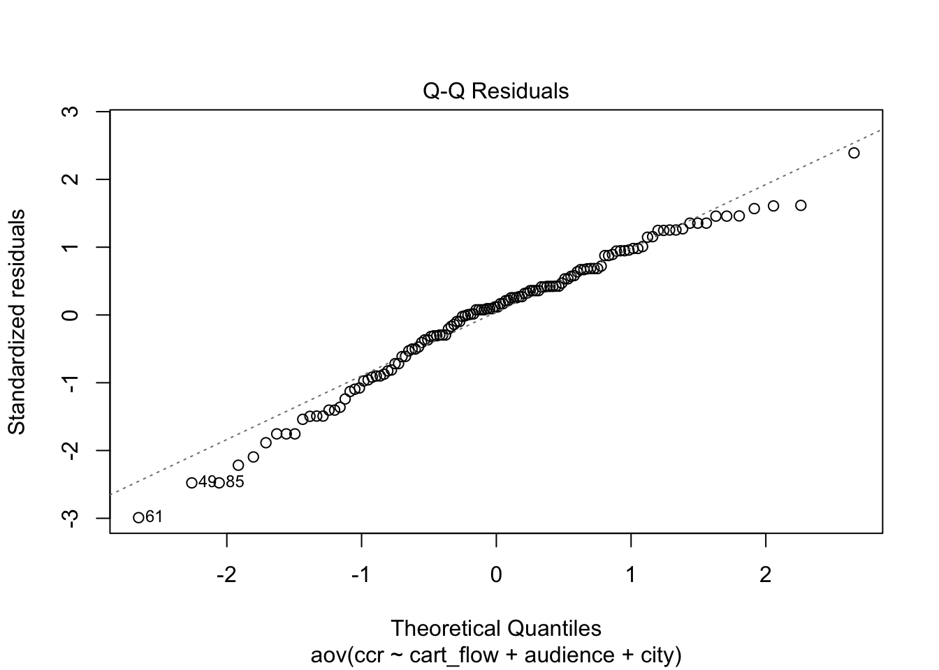
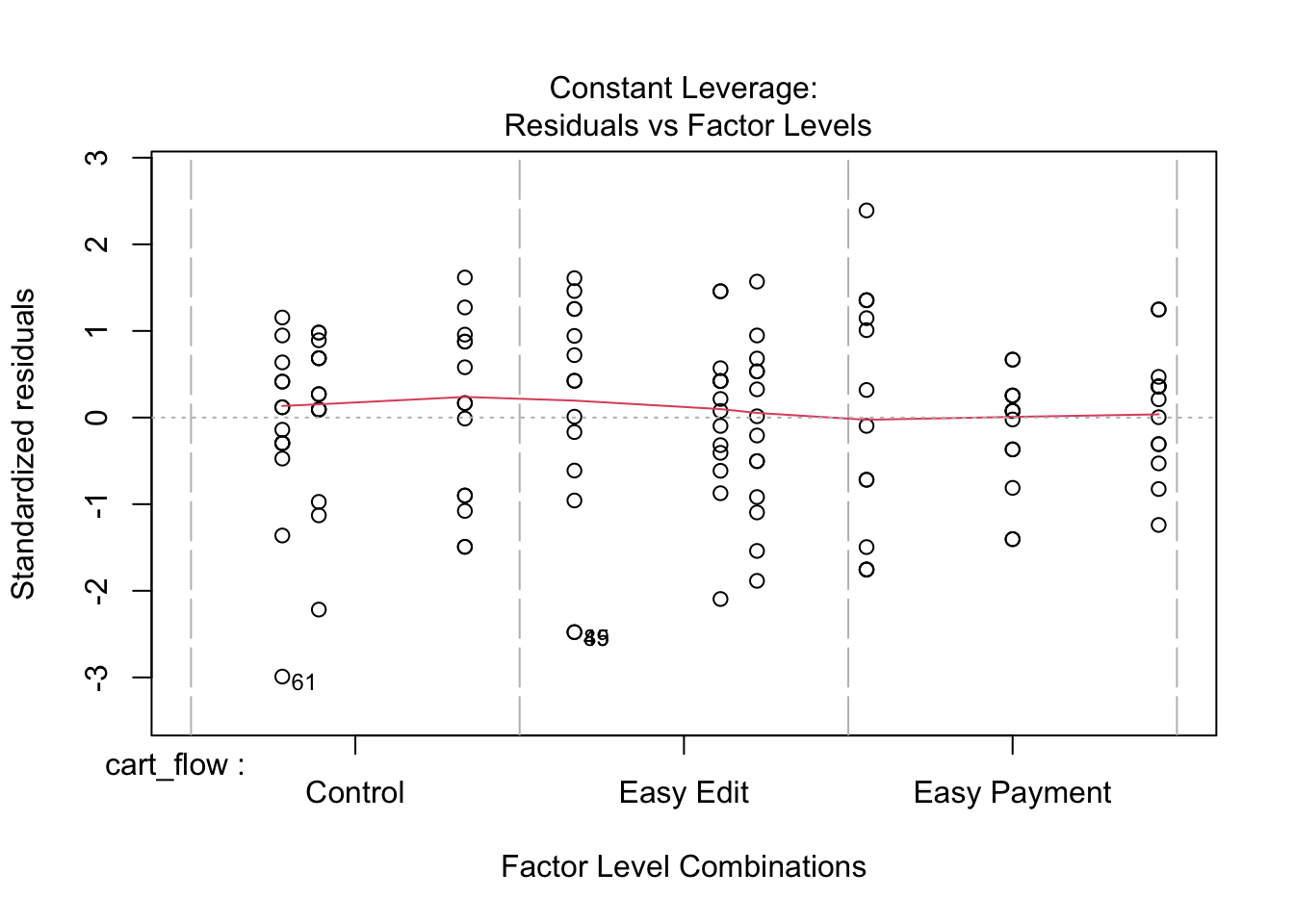
Other Model Assumptions #

A visual check of the model assumptions does not reveal any problems.

Insights #

We can explore the magnitude of the effects from each shopping cart flow by creating a linear model from these data, beginning with the simplest model $\text{CCR}\sim {\tau }_k$, for the treatment factor alone:

 1
 2
 3
 4
 5
 6
 7
 8
 9
10
11
12
13
14
15
16
17
18
19

## 
## Call:
## lm(formula = ccr ~ cart_flow, data = cart_day_summary)
## 
## Residuals:
##      Min       1Q   Median       3Q      Max 
## -0.50383 -0.10348  0.00867  0.12951  0.34201 
## 
## Coefficients:
##                       Estimate Std. Error t value Pr(>|t|)    
## (Intercept)            0.59247    0.02783  21.286  < 2e-16 ***
## cart_flowEasy Edit     0.11136    0.03936   2.829  0.00545 ** 
## cart_flowEasy Payment  0.06553    0.03936   1.665  0.09853 .  
## ---
## Signif. codes:  0 '***' 0.001 '**' 0.01 '*' 0.05 '.' 0.1 ' ' 1
## 
## Residual standard error: 0.1804 on 123 degrees of freedom
## Multiple R-squared:  0.06169,	Adjusted R-squared:  0.04643 
## F-statistic: 4.043 on 2 and 123 DF,  p-value: 0.01992

Here, we see the estimate for the Intercept (control group) of 0.5925 is very much what we expect given the prior month’s data. The Easy Payment cart flow of 0.0655 has just exceeded our MDE, while the Easy Edit cart flow of 0.1114 is slightly more than double.

Digging deeper to view the full model $\text{CCR}\sim {\alpha }_i+{\beta }_j+{\tau }_k$, we now see variance partitioned across the different groups in the LSD:

 1
 2
 3
 4
 5
 6
 7
 8
 9
10
11
12
13
14
15
16
17
18
19
20
21
22
23

## 
## Call:
## lm(formula = ccr ~ city + audience + cart_flow, data = cart_day_summary)
## 
## Residuals:
##      Min       1Q   Median       3Q      Max 
## -0.48091 -0.09506  0.01909  0.10904  0.38451 
## 
## Coefficients:
##                        Estimate Std. Error t value Pr(>|t|)    
## (Intercept)            0.549964   0.039005  14.100  < 2e-16 ***
## cityIstanbul          -0.062937   0.036111  -1.743  0.08394 .  
## cityKraków             0.097610   0.036111   2.703  0.00788 ** 
## audienceRegular        0.006557   0.036111   0.182  0.85622    
## audienceResponder      0.086279   0.036111   2.389  0.01845 *  
## cart_flowEasy Edit     0.111359   0.036111   3.084  0.00254 ** 
## cart_flowEasy Payment  0.065526   0.036111   1.815  0.07211 .  
## ---
## Signif. codes:  0 '***' 0.001 '**' 0.01 '*' 0.05 '.' 0.1 ' ' 1
## 
## Residual standard error: 0.1655 on 119 degrees of freedom
## Multiple R-squared:  0.236,	Adjusted R-squared:  0.1975 
## F-statistic: 6.127 on 6 and 119 DF,  p-value: 1.276e-05

For example the Intercept now represents just the customers in Hamburg in the Other audience segment. This group has a slightly lower CCR at 0.55 but our model shows us that we still expect the significant increase in CCR from the new versions of cart flow.

Conclusions #

We presented Latin Square Designs as an efficient way to run A/B tests while controlling for two known sources of variance. This method increases efficiency relative to a Complete Randomized Design. At the same time, it allows you to reduce the number of experimental samples while maintaining statistical power.

Our real-world example, an optimization for an e-commerce application, tested two potential improvements to the shopping cart flow, blocking over geographical and customer segments factors. It ran for two weeks and yielded a useful insight about which of the improvements to prioritize. Ultimately, both improvements could be deployed in quick succession, avoiding the opportunity cost of running separate, non-concurrent A/B tests.

The relative efficiency score of 1.1882 tells us that the variance was reduced by 15.84%, compared to the CRD. In addition, we also gained by the threefold decrease in the number of customers who needed to participate in the test, two thirds of whom saw a new version of the cart flow. This represents a huge reduction on the risk to these conversion opportunities.