Analysing SaaS Trial to Subscriber Conversions - Part 1 - Going Beyond the Binary Outcomes with Survival Analytics
Last Updated:
Table of Contents
Series Introduction #
This is part one of a series on using Survival Analysis techniques for Product Management. Survival models excel at analyzing time-dependent events where timing matters as much as the outcome itself. Unlike time series analysis that tracks metrics evolving over time (and requires data collected at regular time intervals), survival analysis is event-based and asks a different question: when will something happen, and what influences that timing?
The applications span the entire product lifecycle. A few examples include:
- predicting feature abandonment during onboarding
- modeling churn patterns for lifetime value calculations
- optimizing A/B test duration
- analyzing subscription upgrade timing
- determining optimal re-engagement moments
Each scenario involves understanding not just whether an event occurs, but when it’s most likely to happen and what accelerates or delays that moment.
What makes survival analysis particularly elegant is how it handles incomplete information. When users haven’t yet converted or churned, traditional analytics sees missing data. Survival models see valuable information about persistence and decision-making patterns. The framework naturally accommodates both completed journeys and those still in progress at the end of the trial period, extracting insights that conventional funnel analysis simply cannot capture.
In part one, we’ll introduce a common scenario in product management; the trial-to-conversion journey. With the context in place, we’ll look at essential theoretical fundamentals and end this post with the first step of a much deeper analysis.
Future posts will build on this foundation with stratified estimation and comparison between the groups, and go on to advanced use cases such as time-dependent analyses that track how changing customer behavior, and external events and interventions can influence conversion probability in real-time.
Introduction #
Survival analysis has morbid origins – tracking ’time to death’ in clinical trials. The terminology feels grim: “hazard rates,” “time to failure,” “censored observations.” But flip the script to ’time to success’ and these insights become pure gold for product teams.
The mathematics stay the same, but the mindset transforms everything:
- Customer drops out early? That’s not missing data – it’s product-market fit intelligence
- Converts on day 40 vs day 10? That signals problems with onboarding effectiveness and operational costs
Traditional analytics asks “who converted?” Survival analysis asks “when do they convert, and what accelerates that moment?”
The difference is profound. You can separate controllable factors (onboarding sequences, CS outreach timing) from uncontrollable ones (industry vertical, company size), revealing the critical difference between customers who need more time versus those actively walking away. These insights unlock operational efficiency that directly impacts your bottom line.
As usual, the R code held out for brevity and echoed at the end of the post.
Just Enough Theory #
As usual, I want to give a sense of what’s happening under the hood without drowning in theory. Here’s a very brief primer on how Survival Analysis works.
The Survival Function: S(t) #
The survival function represents the probability that an event (in our case, conversion) has not occurred by time t:
$$ S(t) = P(T > t) $$
where \(T\) is referred to as the time to failure in traditional Survival Analysis but in out context is the time to conversion. For trial customers, \(S(t)\) tells us the probability that a customer hasn’t yet converted by day \(t\). If \(S(t)\) remains high for long, our trials are longer and we take a hit for ongiong operational costs of running the free tier and possibly losing out to the competition.
In our business oriented context, we’re rather more interested in \(1 - S(t)\), the cumulative probability of success/conversion. I’ll refer to this flipped view as the Conversion Momentum Curve.
The Hazard Function h(t) #
This is the most theoretical element we’ll deal with but it’s useful to understand. The hazard function represents the instantaneous risk of conversion at time t, given survival (non-conversion) up to that point:
$$
h(t) = \lim_{\Delta t \to 0} \frac{P(t \leq T < t + \Delta t | T \geq t)}{\Delta t}
$$
and it tells us the probability with which event \(T\) takes place in the instant after time \(t\).
Estimating the hazard function is essential for comparing strata - in our case, it could be customers’ industry vertical or acquisition channel. Given an assumption that the ratio between \(h(t)\) for the strata remain constant over time, it is possible to make statistical claims about any differences.
The Cumulative Hazard (CumHaz) Function H(t) #
The cumulative hazard function represents the total accumulated risk (in our case of conversions, risk is a good thing) from the start of the trial up to time t:
$$
H(t) = \int_0^t h(u) du
$$
In our business context, we can think of \(H(t)\) as the Purchase Decision Momentum that has built up over the trial period. This helps us understand:
- How conversion results accumulate over time.
- Fluctuations in this conversion pressure, perhaps as a result of our customer success interventions.
The cumulative hazard provides a clearer picture of differences between customer segments than the instantaneous hazard rate alone.
Relationship Between Survival and Hazard #
There is a direct relationship that links Survival and Hazard functions via the CumHaz function, making it easy to switch perspectives:
$$ S(t) = \exp(-H(t)) $$
Non-parametric Estimators #
For distribution free estimation learned directly from data, there are methods for both \(\hat{S}(t)\) and \(\hat{H}(t)\) by counting at risk (not yet converted) units at the time \(t\) of every event.
The Kaplan-Meier Estimator for Survival Function Estimation #
$$ \hat{S}(t) = \prod_{t_i \leq t} \left(1 - \frac{d_i}{n_i}\right) $$
where:
\(d_i\)= number of events (conversions) at time\(t_i\)\(n_i\)= number of customers at risk just before time\(t_i\)
Kaplan-Meier Confidence Intervals #
The standard errors are calculated using Greenwood’s Standard Error formula:
$$ SE[\hat{S}(t)] = \hat{S}(t) \sqrt{\sum_{t_i \leq t} \frac{d_i}{n_i(n_i - d_i)}} $$
and these values are stabilised into the zero-one interval using Log-Log transformation:
$$ \hat{S}(t)^{e^{(\pm z_{\alpha/2} \cdot SE[\ln(-\ln(\hat{S}(t)))])}} $$
The Nelson-Aelen Estimator for CumHaz Function Estimation #
We can estimate the CumHaz function directly as well.
$$ \hat{H}(t) = \sum_{t_i \leq t} \frac{d_i}{n_i} $$
Scenario: Analysing SaaS Trial-to-Subscriber Conversion #
When you’re running a SaaS business with a 6-week free trial, the question isn’t simply “did they convert or not?” It’s far more nuanced.
At our e-commerce customer engagement platform, we help online retailers track their customer behavior, optimize product recommendations, and boost lifetime value. This all happens on a per-product basis. That is, we count each enrolled product as a conversion, while many products can come from each billed customer.
So we’ve become pretty astute at analysing our own trial-to-conversion processes. And this revealed something crucial: timing matters as much as the outcome itself.
Every day that a prospect remains in trial without converting carries real costs. Our infrastructure supports thousands of free-tier users analyzing their customer data, our customer success team schedules personalized demos and sends targeted outreach.
This business model has consequences; delayed conversions mean delayed revenue in a competitive market. When a retailer finally converts after 5 weeks instead of 2 weeks, we’ve absorbed additional operational costs while potentially losing deals to competitors who moved faster. Traditional conversion analysis treats late converters the same as early ones, but from both a cost and revenue perspective, they’re fundamentally different.
Using Survival Analysis on this data provides invaluable insight. When prospects go inactive, this isn’t missing data, it’s critical information. When a user actively unsubscribes, we know we lost out to a competing risk that has a time-critical element we can quantify. Most critically, just as you would expect with a logistic model, we can isolate the factors we can control (customer success outreach timing, onboarding flows, feature recommendations) from those we can’t (industry vertical, company size, acquisition channel), with the added benefit of understanding the element of timing.
The result? Actionable insights that directly impact our bottom line and operational efficiency.
What the Data Tells Us at First Glance #
Let’s follow a few good practices and get a sense of the key signals and early insights from our data.
Data Quality #
|
|
|
|
|
|
|
|
|
|
|
|
The data is collected for a random selection of 500 customer accounts who started on the free trial at least 10 weeks prior to today. This means all products that don’t convert will ultimately be censored at day 70 no matter the exact date they started. As part of our regular operations policy, we also put accounts on ice after 6 weeks or 42 days of inactivity to prevent accruing operating costs for mothballed accounts. This cutoff results in earlier censoring for those records. Customers may also unsubscribe altogether. While rare, this event counts as a competing risk:
- They chose one of our competitors.
- They do not see the benefit of using the product.
We can see from the time range that the first conversion within this selection took place after 5.3 days. Our median trial duration date of 46.7 reflects the sampling parameters of the analysis.
Overall Conversions #
|
|
16.2% is close to our prior expectation and is a pretty healthy conversion rate for any SaaS. However, given our niche, we’d hope to do even better with customers in active trials. So we need to deliver a set of actionable insights when we get into the full analysis.
Let’s keep exploring with simple groupings to get a sense of some key drivers.
Conversions by Industry Vertical #
We operate in two industry verticals (homeware and industrial components), so let’s take a quick look for any major differences:
| industry | n | convs | conv_rate | med_time_all | med_time_conv |
|---|---|---|---|---|---|
| homeware | 1589 | 296 | 18.6 | 44.8 | 22.7 |
| industrial | 815 | 94 | 11.5 | 49.7 | 22.5 |
We can see from this table that industrial components customers convert a bit less frequently, but there doesn’t seem to be a difference between the median conversion times. For both metrics, we’d want to find out if these differences are significant, and whether there are any drivers we can control to boost the weaker metric in each case.
Conversions by Customer Acquisition Channel #
We put a lot of product management and marketing effort into content marketing. This is to meet our customers where they are and show by example how our product solves some very specific pain points. There is a much greater CAC and opportunity cost on our content channel, so knowing whether this effort pays off is essential.
| acquisition_channel | n | convs | conv_rate | med_time | med_time_conv |
|---|---|---|---|---|---|
| content | 454 | 89 | 19.6 | 40.0 | 25.4 |
| organic | 770 | 119 | 15.5 | 50.3 | 22.2 |
| paid_ads | 649 | 92 | 14.2 | 52.7 | 22.7 |
| referral | 531 | 90 | 16.9 | 44.5 | 20.9 |
Here we see the conversion rate on the content channel is reassuringly a couple of percentage points higher than other channels. However, the time in trial is slightly longer. This is an interesting signal in the data and if we can clearly identify a driver, we would act. On the flip side, we wouldn’t want to interfere and reduce the effectiveness of this channel.
We also note that paid ads has the lowest conversion rate, while the CAC is also relatively high. This is worth a closer look too.
Crosstabs #
Let’s create a crosstab from the industry vertical and channel dimensions to get a more detailed understanding.
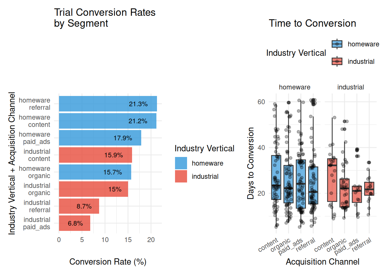
Conversions #
| industry | content | organic | paid_ads | referral |
|---|---|---|---|---|
| homeware | 21.2 | 15.7 | 17.9 | 21.3 |
| industrial | 15.9 | 15.0 | 6.8 | 8.7 |
It seems that industrial customers acquired by paid ads and referrals are the least likely to convert, while these same channels perform very well in the homeware vertical. This early insight aligns pretty well with the product manager’s domain experience: these customers have very different profiles. Industrial customers that convert were more directed in their research and didn’t tend to click on sponsored links. Similarly, their procurement processes are stricter and more hierarchical. Network effects are less likely to break through.
Median Time to Convert #
| industry | content | organic | paid_ads | referral |
|---|---|---|---|---|
| homeware | 23.5 | 22.2 | 24.2 | 20.6 |
| industrial | 32.2 | 22.1 | 21.1 | 21.7 |
We’re also seeing a really long median conversion time relative to the other groups for industrial/manufacturing customers who were acquired through content marketing. This was not at all expected but we start with a working hypothesis that these customers are much more deliberative in their decision-making, given the depth of engagement early in the funnel.
Visual Summary #
As always, a picture tells a thousand words when it comes to data analysis. Here we see an intuitive view of these preliminary EDA findings
Other Metrics #
We have a few other dimensions such as customer region (we sell into six different countries), and the initial engagement level in the trial. Then there are time dependent metrics, such as ongoing engagement. To keep this post from ballooning, we’ll get more into those weeds in the forthcoming posts.
Tracking the Customer Journey: From Trial Day One to Decision Day #
Now we move from exploratory static snapshots to dynamic storytelling using Survival Analysis. The classic Kaplan-Meier estimation method lets us track how conversion probability evolves day-by-day throughout the trial period.
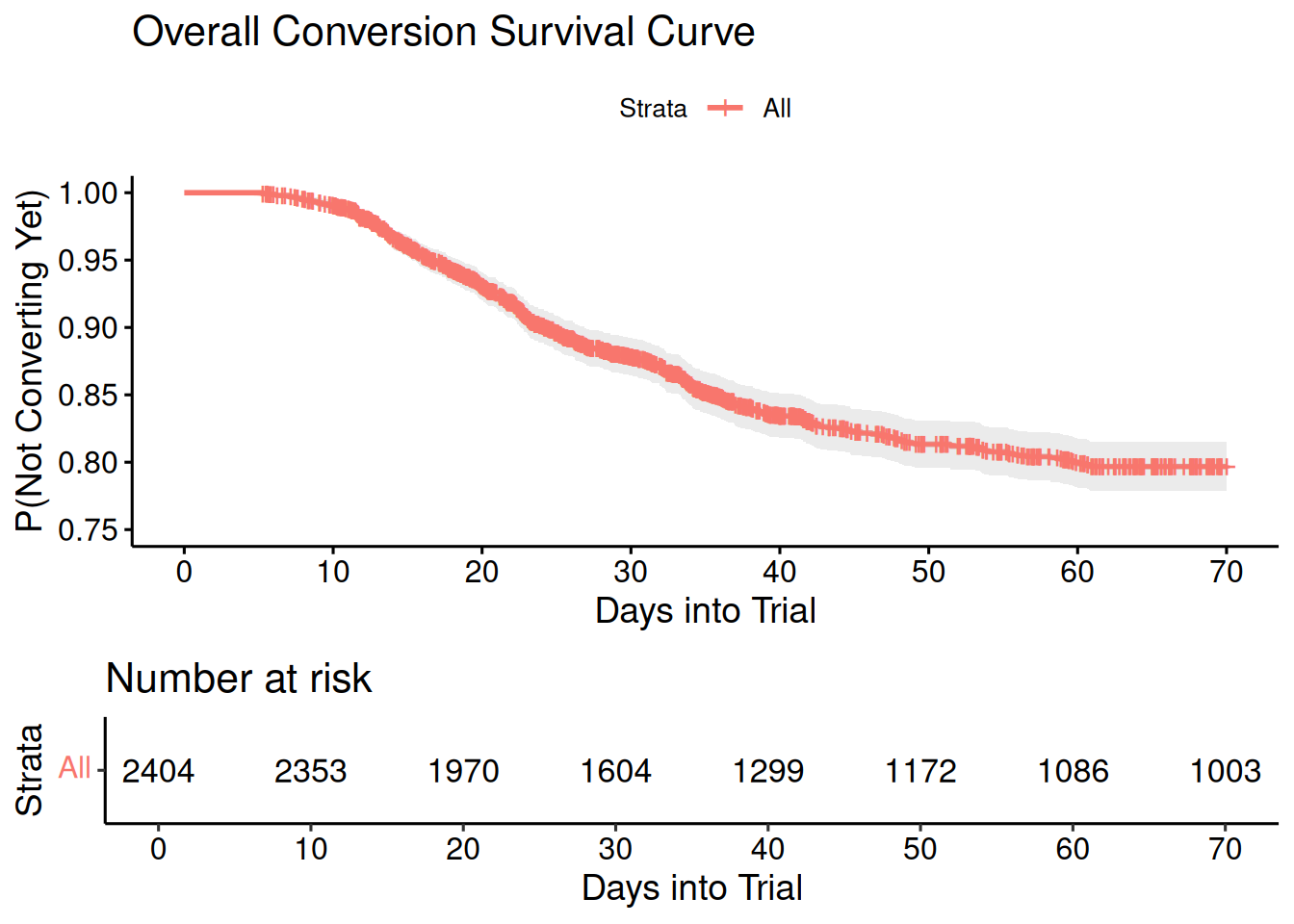
Reframing the Survival Narrative With Overall Conversions #
We’ll look first at a traditional survival curve, which actually measures the probability of not converting. The survival curve has a few key features. It always begins at 1.0, with all individuals in the study at risk. It is monotonically falling because once an individual converts, they never rejoin the at-risk pool. The small vertical bars on the curve represent conversion and censoring events. On the above curve, they are rather dense but we’ll see later with stratified curves that this can be more informative.
However, I want to flip these plots upside-down to create conversion momentum curves, showing a more intuitive cumulative probability of conversion over time. We also don’t want to talk about the number of individuals still “at risk” but rather the number of products “yet to convert.”
This reframing transforms survival analysis from a clinical mindset into a growth mindset.
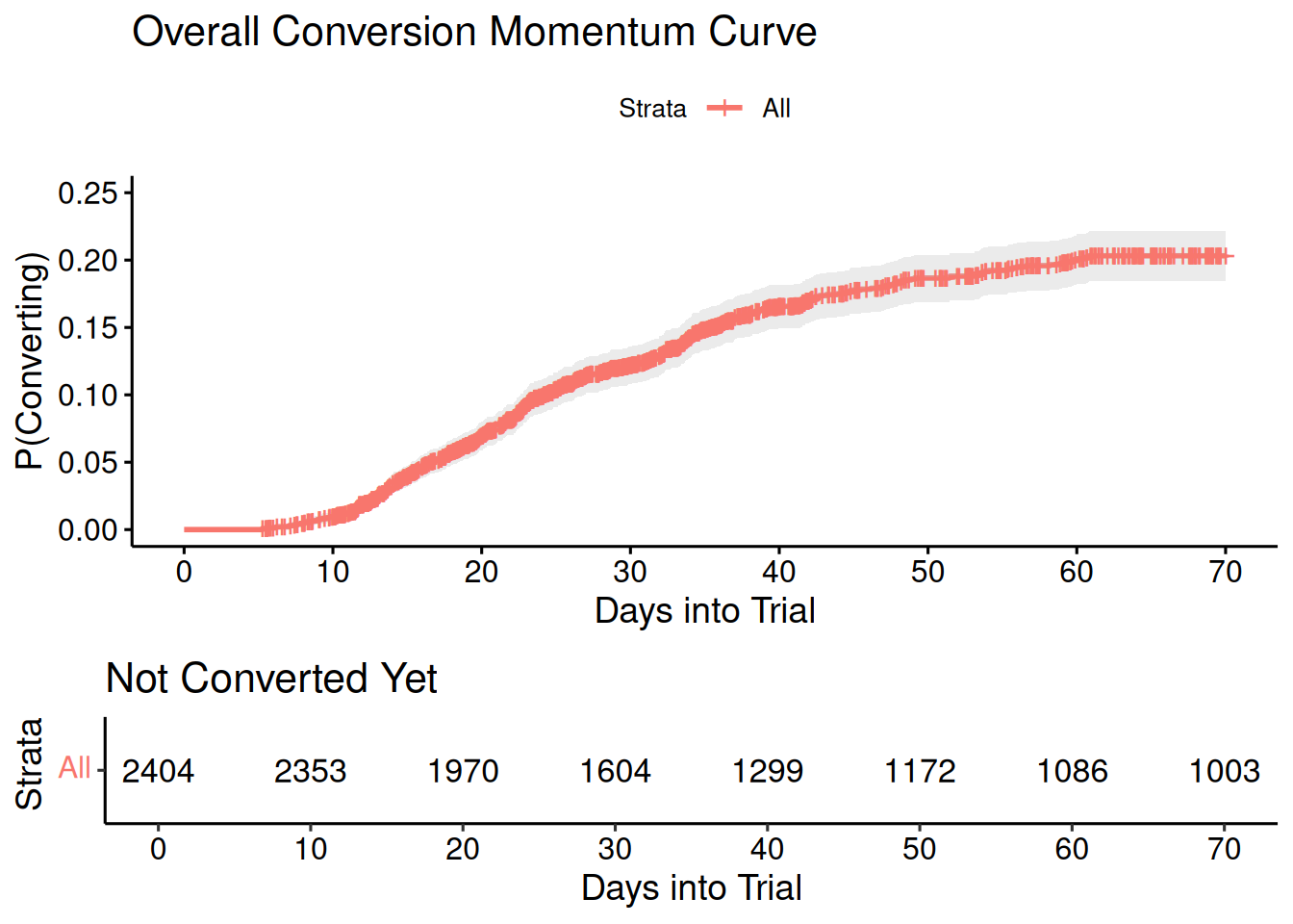
As we go deeper with the investigation, we will stratify the curves to tell the story of how different customer segments build momentum toward their purchase decision, revealing not just who converts, but when conversion accelerates and what drives that critical moment of commitment.
Redefining Meaningful Milestones: From Medians to Early Indicators #
Traditional survival analysis relies heavily on the median survival time. This is the point where 50% of the population has experienced the event. It’s a natural milestone that splits the data in half and provides an intuitive benchmark for comparison.
But here’s the challenge: our SaaS trial data shows only 16% conversion rates, meaning the survival curve never drops below 84%. The median simply doesn’t exist in our dataset – mathematically.
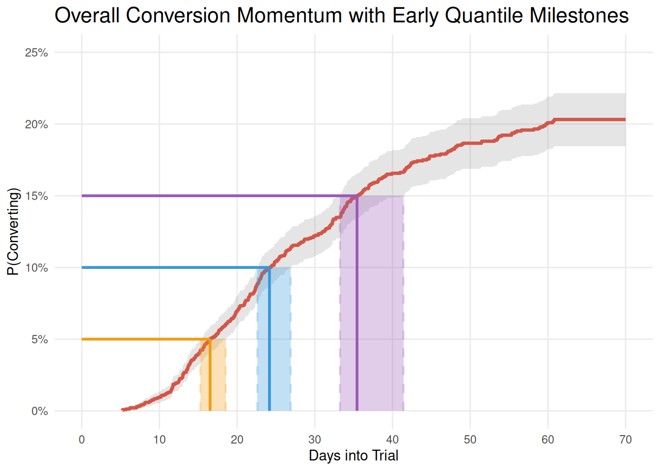
This reality forces us to adapt our approach. We can focus on the quantiles that actually occur within our business timeframe – the 5th, 10th, and 15th percentiles of conversion timing. These early milestones capture the behavior of customers who do convert, revealing actionable insights about when momentum builds and decisions crystallize, rather than chasing statistical conventions that don’t match our business reality.
| quantile | days | lower | upper |
|---|---|---|---|
| 0.05 | 16.5 | 15.3 | 18.5 |
| 0.10 | 24.2 | 22.6 | 26.9 |
| 0.15 | 35.4 | 33.2 | 41.4 |
This is a bit of a mouthful to explain, but in essence, it’s just a question of drawing a horizontal line from the required conversion rate, and reading the value at the x-axis where the line intersects the curve (and it’s confidence intervals). This is easier to understand with the following annotated plot.
Summary #
We’ve introduced Survival Analysis as an extremely useful tool in the Product Management life cycle. We covered the fundamental theoretical principles, including non-parametric estimation (learning from timed event data). Then we introduced a specific scenario; trial-to-conversion, explored our data set and took the first step in modeling and interpreting the Survival curve, through the lens of Product Management.
In the next post, we’ll estimate new survival curves, stratified by our key factors, such as vertical and channel, to compare Survival estimates between groups.