Analysing SaaS Trial to Subscriber Conversions - Part 2 - Comparing Groups with Stratified Analysis

Introduction #

You can read the Series Introduction here

In the previous post, we saw how a Survival curve can be reframed as a Conversion Momentum Curve (CMC), giving us a way to esitmate when (counting in days from the start of a free trial period) we will reach conversion rate milestone of e.g. 5%, 10%, or 15% of free trial users. This is useful information because anything we can do to shorten the free trial period for our SaaS product offsets our fixed operating costs with new revenue.

We saw that our overall CMC looks like this:

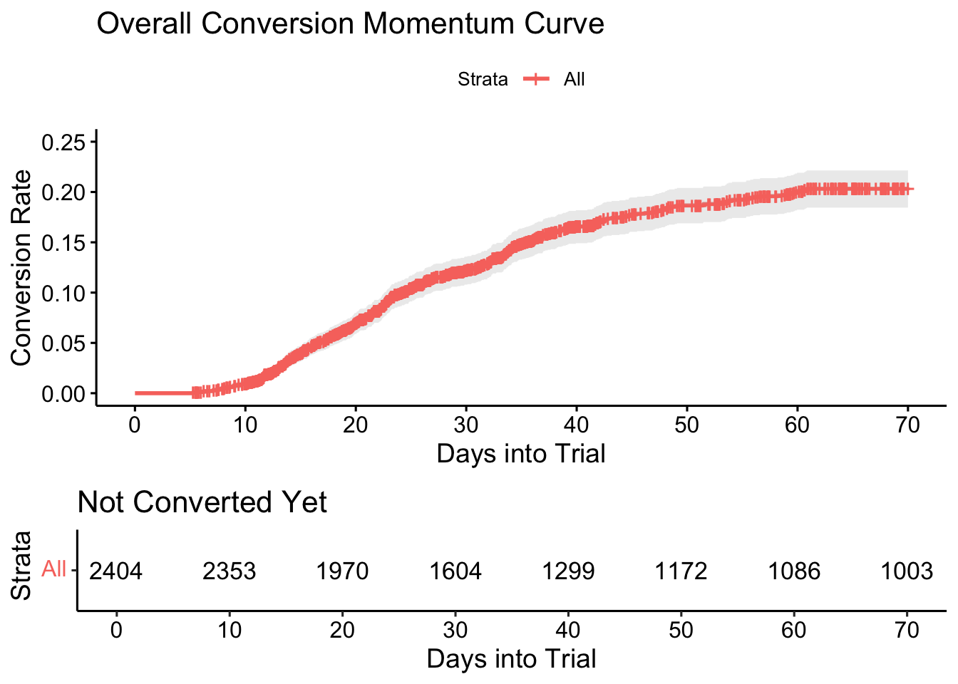
This curve shows us the cumulative conversion rate at time $t$ (days) and gives us a sense of how the conversion rate evolves over the time spent in the free-trial period.

In this follow-up post, we use the standard KM-estimator method to estimate a non-parametric CMC and analyse differences between groups according to industry, acquisition channel, and geographic sales region. In Survival Analysis, this is called stratified estimation and, with certain assumptions, we can make inferences and hypothesis tests about the differences.

We consider customer invariant data that is already decided at the start of the free trial period that we cannot intervene on. We can only react to it. We track many other customer variables, such as the frequency with which they login and the customer success calls that we conduct with them. These types of variables are time dependent, just like the conversion event itself. The time they take place can have a profound effect on increasing or decreasing the likelihood of conversion. This requires a different analysis, which we won’t cover in this post. Look out for the next one if you are interested.

Industry Verticals #

We also saw that there were some apparent differences in the raw numbers for the two main industry verticals in which we operate: Homeware and Industrial Components

Let’s see how these differences manifest in the CMC analysis:

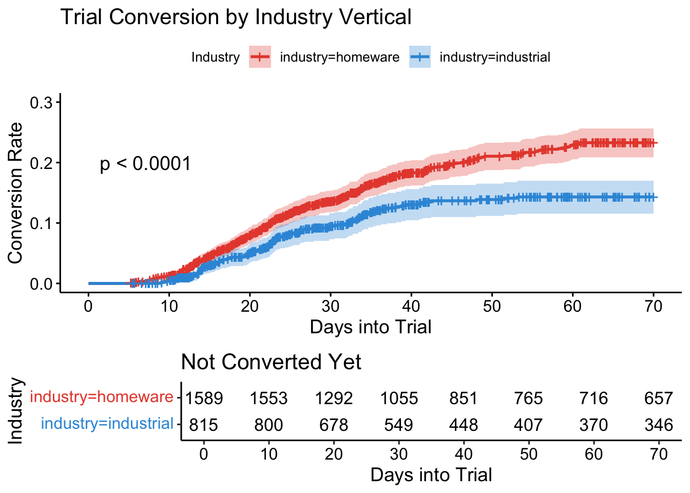
This chart gives us a very clear indication that these two curves are different. Very early on, the event lines separate and the confidence intervals no longer overlap. The charting code runs a Log-rank test in the background and p-value of this test is displayed. For completeness, we can also show the full Log-rank test table, which is based on a ${\chi }^2$ test statistic:

1
2
3
4
5
6
7
8

## Call:
## survdiff(formula = surv_obj ~ industry, data = survival_data)
## 
##                        N Observed Expected (O-E)^2/E (O-E)^2/V
## industry=homeware   1589      296      257      6.04      17.7
## industry=industrial  815       94      133     11.62      17.7
## 
##  Chisq= 17.7  on 1 degrees of freedom, p= 3e-05

Acquisition Channels #

Previously, we also so some crucial differences in the conversion rates per customer acquisition channel. It is essential for us to analyse this more deeply and understand how to optimise our marketing spend.

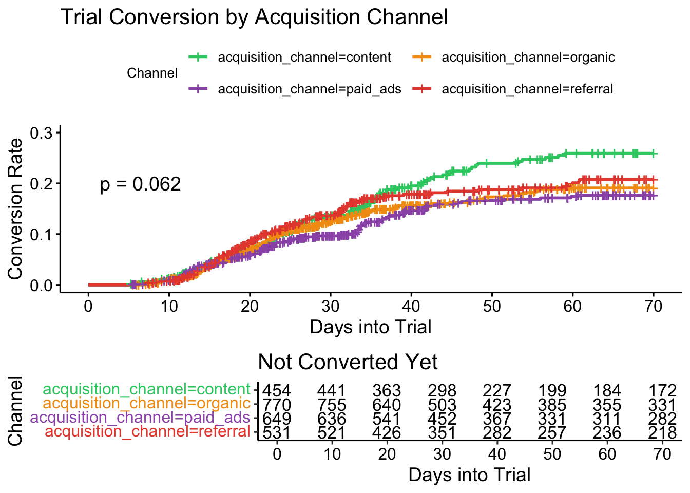
The confidence intervals have been omitted because there is a lot of overlap, which is somewhat messy with four overlapping curves.

 1
 2
 3
 4
 5
 6
 7
 8
 9
10

## Call:
## survdiff(formula = surv_obj ~ acquisition_channel, data = survival_data)
## 
##                                N Observed Expected (O-E)^2/E (O-E)^2/V
## acquisition_channel=content  454       89     71.3     4.390     5.374
## acquisition_channel=organic  770      119    125.7     0.362     0.534
## acquisition_channel=paid_ads 649       92    107.7     2.300     3.179
## acquisition_channel=referral 531       90     85.2     0.270     0.345
## 
##  Chisq= 7.3  on 3 degrees of freedom, p= 0.06

The results here are rather nuanced. With a p-value of 0.062, the evidence against the null hypothesis of no difference between the curves is borderline or weak. We also see the event lines crossing in some places, indicating either no difference, or that an assumption of constant proportion between the hazard rates over time is violated.

Nevertheless, we can see visually that the content channel does diverge from the other three more dramatically when $t>40$, which supports what we saw in the raw numbers. In a situation like this, it can be more valuable to run a pairwise comparisons test.

1
2
3
4
5
6
7
8
9

## # A tibble: 6 × 4
##   Channel1 Channel2 p_value p_adjusted
##   <chr>    <chr>      <dbl>      <dbl>
## 1 organic  paid_ads  0.463      0.463 
## 2 organic  content   0.0457     0.137 
## 3 organic  referral  0.44       0.463 
## 4 paid_ads content   0.0094     0.0564
## 5 paid_ads referral  0.151      0.301 
## 6 content  referral  0.260      0.389

These results suggest that the differences between content vs paid ads and content vs organic channels are significant.

Industry and Channel Interactions #

We can, of course cross-tabulate and stratify on both items to see differences in channel performance across vertical.

 1
 2
 3
 4
 5
 6
 7
 8
 9
10
11

## # A tibble: 8 × 6
##   industry   acquisition_channel     n conversions conversion_rate median_time
##   <chr>      <chr>               <int>       <dbl>           <dbl>       <dbl>
## 1 homeware   referral              348          74            21.3        42.1
## 2 homeware   content               316          67            21.2        40.5
## 3 homeware   paid_ads              429          77            17.9        47.1
## 4 homeware   organic               496          78            15.7        52.8
## 5 industrial content               138          22            15.9        38  
## 6 industrial organic               274          41            15          45.5
## 7 industrial referral              183          16             8.7        50.8
## 8 industrial paid_ads              220          15             6.8        64.6

The summary table in the previous post (reproduced here) showed some really obvious differences for the nested results and we had a rational business explanation for this situation: Paid search and referrals do not penetrate well to the right kind of customers in the Industry vertical, who seem to be more intentional in their search for our product.

Let’s flip back to a traditional orientation of the survival curve to understand the impact of this on our operations.

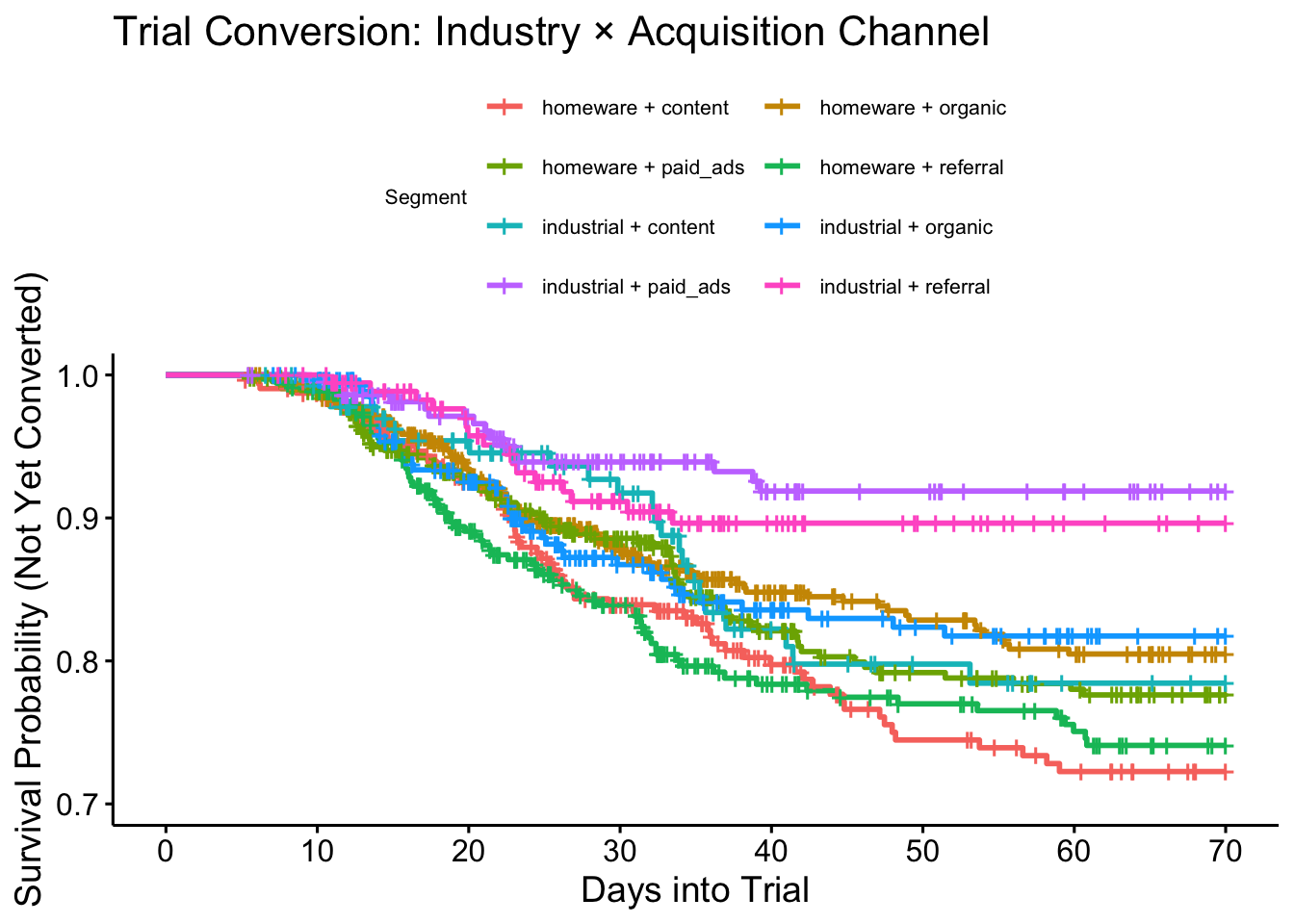
Here we see the conversions for referrals end after around $t>30$ and for paid search after $t>40$. The event line flattens out entirely. With this knowledge, we can adjust our offer to customers acquired through these channels and shorten the free trial period, cutting these operating costs much sooner.

Another perspective that we looked at in the previous post was conversion rate milestones. That is, an estimate of the free-trial period that will yield a given conversion rate. This is an adapation of the median survival time to use different quantiles. For example, the 0.1 quantile gives the number of days at which we still have 90% of the trial users unconverted. NA shows where the population never drops below this level.

In the above table we can see that the content marketing channel in the industrial vertical doesn’t look any better than the referral channel but we know this is not the case from the survival curve. In fact these two curves cross after the 30 day mark, demonstrating very different behaviours with many more customers converting after a longer period in trial.

We can also consider flipping this milestone to an estimate of the conversion rate or proportion of unconverted (survival) after specific periods in free-trial. This is useful to check how much value is left “on the table” when we end the trial periods too early.

Here we see that waiting until 45 days delivers an additional 10% conversion for this channel. This delivers very significant business value!

Geographic Sales Region #

Let’s take a look at the last customer invariant, which is of limited interest because there aren’t many levers we can pull around the way cultural and local business factors affect purchasing behaviours.

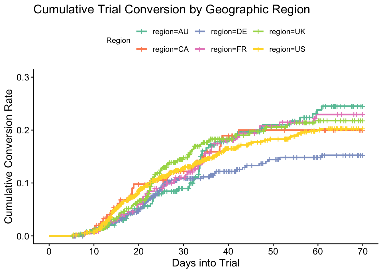
We see most of the regions are pretty similar, other than the German (DE) market which begins to lag behind the others after 30 days. Australia is also interesting because it picks up pace around that time and crosses (overtakes) all the other regions conversion rates to take the top spot by the end of the ten week cut off. People in this market really take their time to become familiar with the product for the first month or so and do not rush into making a decision but the product is quite popular in the end.

Let’s run the pairwise Log-rank tests to look for significant differences.

 1
 2
 3
 4
 5
 6
 7
 8
 9
10
11
12
13
14
15
16
17
18

## # A tibble: 15 × 4
##    Region1 Region2 p_value p_adjusted
##    <chr>   <chr>     <dbl>      <dbl>
##  1 UK      CA       0.742       0.972
##  2 UK      US       0.565       0.972
##  3 UK      FR       0.953       0.972
##  4 UK      AU       0.942       0.972
##  5 UK      DE       0.0296      0.227
##  6 CA      US       0.972       0.972
##  7 CA      FR       0.797       0.972
##  8 CA      AU       0.688       0.972
##  9 CA      DE       0.196       0.589
## 10 US      FR       0.657       0.972
## 11 US      AU       0.531       0.972
## 12 US      DE       0.0538      0.227
## 13 FR      AU       0.884       0.972
## 14 FR      DE       0.0605      0.227
## 15 AU      DE       0.038       0.227

We see that all the comparisons with DE are significantly different when considering the non-adjusted p-values but not when the tests are adjusted for the multiple comparisons. No other significant differences are found. The insights gained may be used to modify incentives within the German sales process.

Customer Engagement Level #

As mentioned, this variable represents the initial feature selected by the customer during their initial onboarding. This is an ordinal factor with four levels because we don’t go so far as analyzing which of the four main features are activated. In fact, we simply convert this to a binary factor for Low Engagement (< 3 features) or High Engagement (>= features).

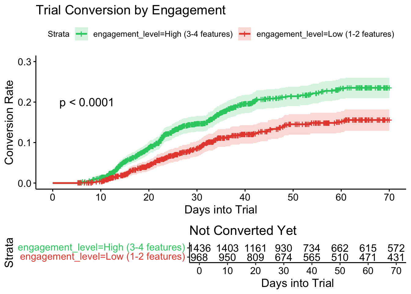
We see that the customers with a high initial engagement have a significantly higher conversion rate, certainly from around day 15 onward. Note that we cannot say with any certainty what the causal direction is. Are these customers already interested in all the features and are therefore more likely to convert, or does early exposure to all the feature convince them. It is not within the capability of this type of analysis to say with any certainty.

The Log-rank test result is also shown.

1
2
3
4
5
6
7
8

## Call:
## survdiff(formula = surv_obj ~ engagement_level, data = survival_data)
## 
##                                         N Observed Expected (O-E)^2/E (O-E)^2/V
## engagement_level=High (3-4 features) 1436      272      228      8.51      20.5
## engagement_level=Low (1-2 features)   968      118      162     11.97      20.5
## 
##  Chisq= 20.5  on 1 degrees of freedom, p= 6e-06

Summary and Conclusion #

In this post, we used the KM-Estimator to estimate a “flipped” survival curve, effectively $1-S(t)$. This is more intuitive when discussing cumulative free-trial conversions. We carried out the technique to stratify our curves by multipled customer invariant data. These are factors that are already determined before the trial and won’t change, such as the geographich sales region and the customer acquisition channel.

We used a few additional techniques to estimate milestone quantiles: by when will we achieve a certain conversion rate? how much does the conversion rate change between two fixed time points, such as 30 days and 45 days.

We used the Log-rank test (adjusting for multiple comparisons if necessary) to assess statistical significance between the strata.

Over all, with this very straightforward analysis, we were able to gain a lot of business insights that have the potential to reduce operating costs and boost conversions in certain markets.