Non-Parametric Survival Analysis of a Sleep Diary
Last Updated:
Table of Contents
Introduction #
Earlier this month I carried out a parametric survival analysis over a self-generated dataset of my sleep times each day over the previous year. Using the scientific method, of course, I set about the task with a null hypothesis that eating certain food groups for dinner had no effect on my sleep. The findings were indeed very interesting, and I was able to reject the null hypothesis using a parametric regression of the data set using a Weibull survival regression. You can read about that here, so I won’t repeat myself and I’ll skip the exploratory analysis. Just remember, the diagnosis is not great! My median nightly sleep time is 5.84 hours, or 05 hours 50 minutes 34 seconds.
In this post, I take the opportunity to explore the same dataset with a more widely used survival analysis, the non-parametric Kaplan-Meyer estimator. As usual, I’ll differ printing out code until the end, unless there is something interesting to show in context.
The K-M Estimator #
The K-M Estimator is calculated cumulatively at each time point where an event occurs.
$$
\hat{S}(t) = \prod_{\substack{t_i \leq t}}{\left( 1 - \frac{d_i}{n_i}\right)}
$$
where \(n_i\) is the number of observations who have survived up to time \(t_i\), or in my case the number of nights where I would still be asleep, and \(d_i\) is the number of observations who fail at time \(t_i\), or in my case, the number of nights where sleep ends at that elapsed time.
The variance of this estimator is:
$$
\mathrm{var}\left( \hat{S}(t) \right) \approx \left[ {\hat{S}(t)}^2 \right] \sum_{\substack{t_i \leq t}} \frac{d_i}{n_i(n_i - d_i)}
$$
and it is usual to take the complementary log-log transform \(\mathrm{var} \left( \log \left[ -\log {\hat{S}(t)}^2 \right] \right)\) to constrain the confidence intervals between zero and one.
In a typical survival study, there is an additional factor to consider. Survival studies originate in longitudinal studies of people and conditions generally ending in death. Longitudinal studies are prone to individuals exiting the study over time for other reasons than the events under analysis. When an individual exits the study early, their record is said to be right-censored. It is clipped at the point in time when the individual is no longer observed. It is possible to use the information provided by their length of survival during participation, so long as the uncertainty is also taken into account of not being able to observe if/when the event occurs (e.g. death, relapse, or failure in the case of hardware). Right-censored events increase the variance following the end of their time in the study.
To represent the right-censoring in R, you would provide a Boolean vector of equal length as the observations vector into the Surv object. In my sleep diary, however, each observation is a completely measured night’s sleep and so there aren’t any censored observations. To demonstrate the intricacies of this method, I will first construct the univariate estimator, without adding any co-factors, so the formula is given with just a constant (~1).
|
|
|
|
The median sleeping time and 95% confidence intervals are provided by the estimator based on:
$$ \hat{t}_{\mathrm{med}} = \mathrm{inf} \lbrace t : \hat{S}(t) \leq 0.5 \rbrace $$
R makes everything trivial to calculate. The median sleeping time is 05 hours 50 minutes 34 seconds with a lower confidence estimate of 05 hours 38 minutes 35 seconds and an upper confidence interval of 06 hours 05 minutes 49 seconds.
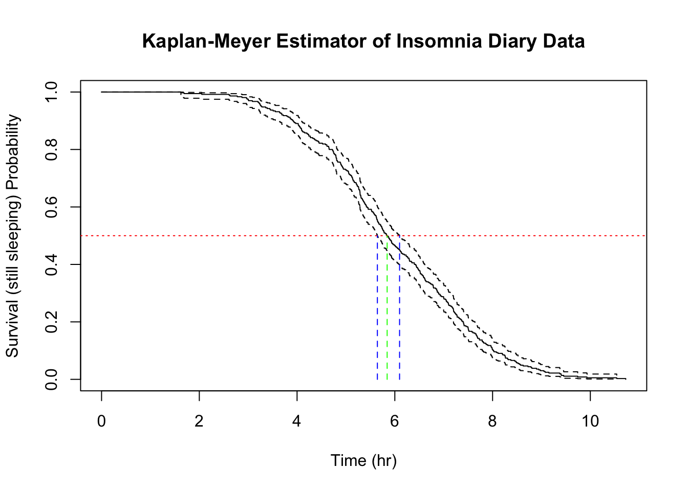
The red (reference) line represent the level where \(\hat{S}(t) = 0.5\) and the green (median) and blue (ci) drop lines show where the reference line intersects with the estimator and its confidence interval.
Typically, survival curves from KM estimators do not look like this. Thanks to the even density of data points (this is essentially a time series), the above plot looks like taking the 365 observations stacked on top of each other in order from the shortest on top to the longest at the bottom. The resulting curve has some similarity to the Weibull curves that I was able to infer using the parametric approach.
Multivariate Analysis #
Categorical Variables #
Non-parametric survival analysis, with it’s roots in clinical trials, is well-developed for comparing two groups and handling perhaps one categorical co-variate with a small number of strata, or one continuous co-variate, but it certainly isn’t common to see the exploratory approach that I used in the previous post on parametric methods.
Sticking to tried and testing methods, I’ll just demonstrate some simple between groups hypothesis testing, using one food trigger at a time. Recall that eating a meal containing cheese for dinner seemed to have a very pronounced effect on me, reducing the median sleep time by about 1 hour 40 minutes when comparing nights when dinner contained none of the analysed food triggers.
I will test the null hypothesis that eating cheese has no effect on sleep times. That is \(H_0 : S_C(t) = S_N(t)\) and the alternative is \(H_A : S_C(t) \neq S_N(t)\) (or \(H_A : S_C(t) < S_N(t)\) for a one-sided test), where \(S_C\) is the survival distribution for cheesy nights, and \(S_N\) for nights with no food trigger. The standard test is the Mantel-Cox test or log-rank test, which tallies a contingency table for treatment (cheese) and control (no food trigger) observations at each event (end of sleep cycle) time. I won’t reproduce the full derivation here but the resulting statistic follows a \(\chi^2\) distribution.
|
|
Evidently, this is a significant result and the null hypothesis is rejected. The effect can be visually analysed with a simple plot.
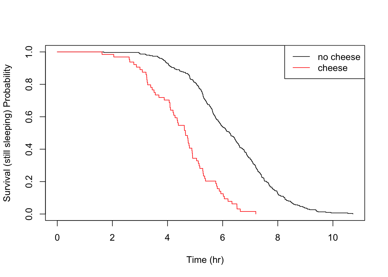
What’s nice about the KM estimator survival curve is that, unlike a parametric distribution, you can clearly see the location of each event, giving you full transperancy over your empiricial data. In a typical survival study, with perhaps only tens of subjects, the piece-wise nature is really clear and locating sudden changes in the distribution is a matter of a quick visual check.
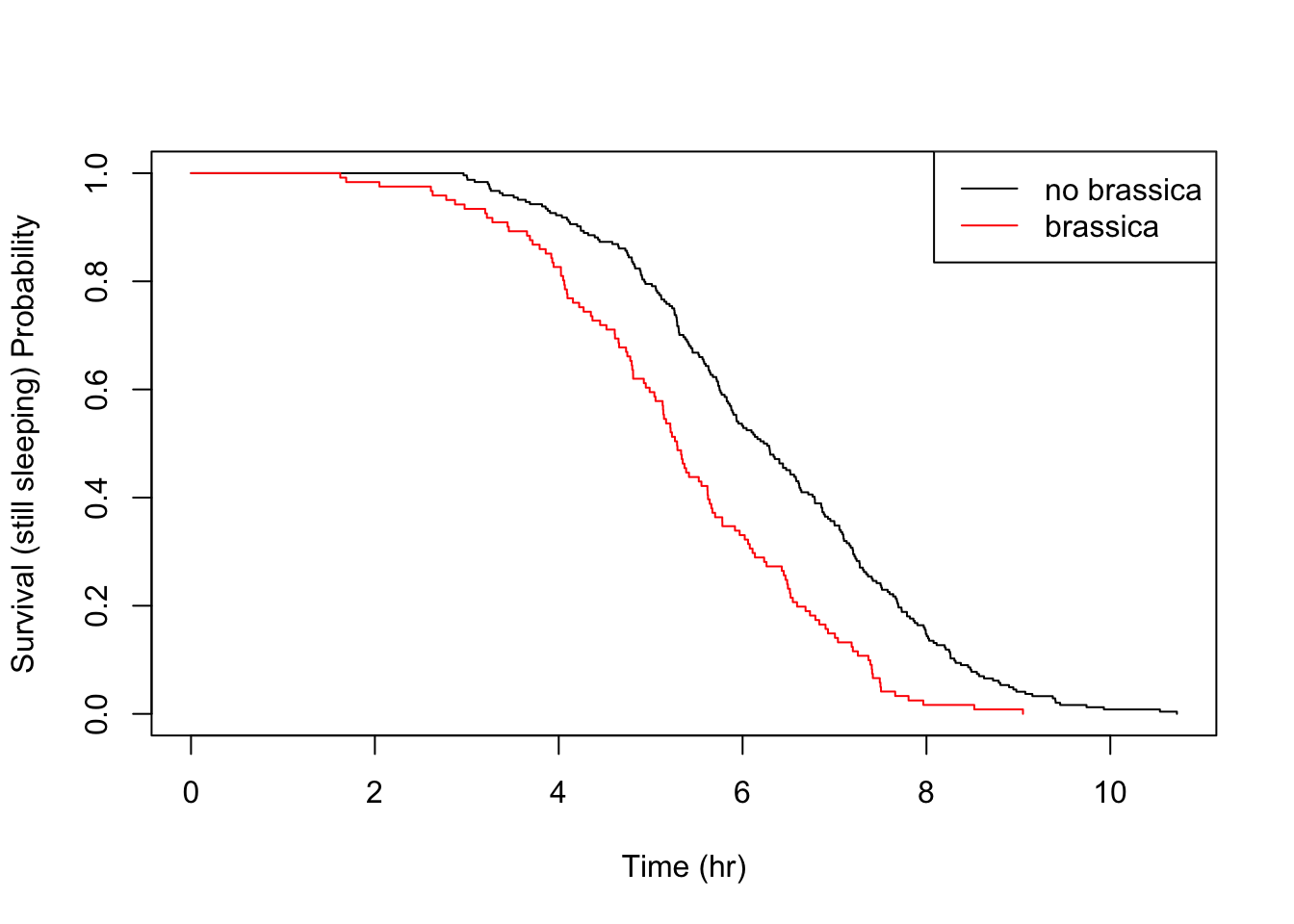
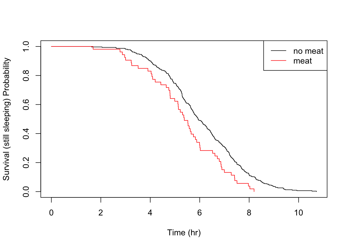
Let’s take a look at the other food triggers.
|
|
|
|
|
|
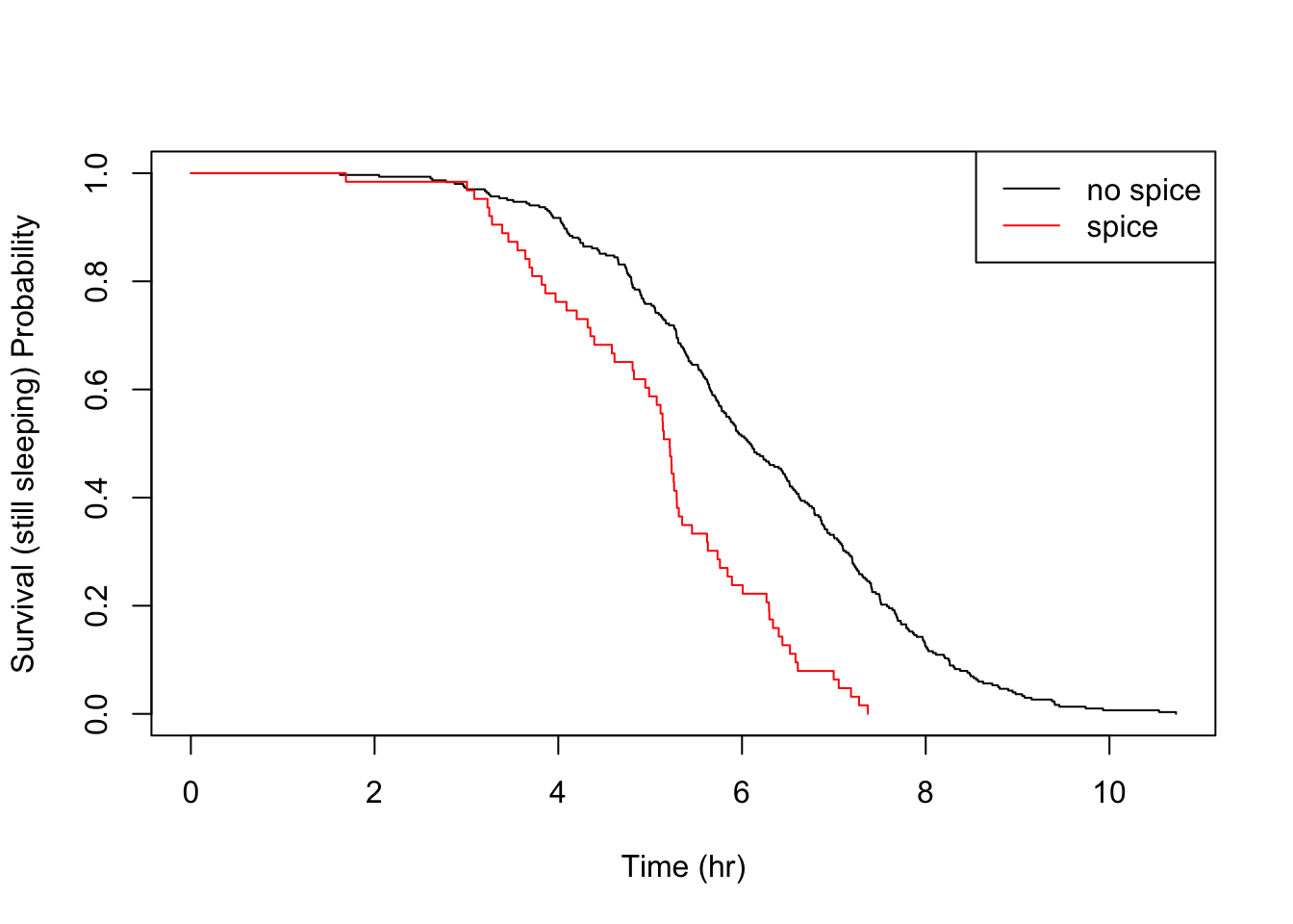
All the above details are consistent with the parametric findings.
Continuous Variables #
In the previous post, by creating autoregressive features from the time sleeping variable, I identified that the sleep time from the night before affected the sleep time for a given night. I assume that there was some physiological pressure to “catch up.” The same was not true for the previous to last night. We can perform a similar investigation non-parametrically.
I haven’t referred to the hazard function \(h(t)\), because I want to keep these posts a bit light on detail, but this is essentially the instantaneous failure rate at time \(t\). It is defined as follows:
$$ h(t) = \lim_{\substack{\delta \rightarrow0}} \frac{P(\mathrm{event_T} | t < T < t + \delta | T > t)}{\delta} $$
where \(P(\mathrm{event_T})\) is the probability of an event happening at instant T within some tiny time increment \(\delta\). There is a mathematical relationship between hazard and survival but it takes a few steps to derive it, so I’ll be a bit hand-wavey here and just say that where \(h(t)\) is high, \(S(t)\) is falling fast.
Analysis of hazard functions is done by Cox’s Proportional Hazards, which uses a log-likelihood statistic and can be used for survival regression. The coefficients of a proportional hazards regression analysis follow a normal distribution and so can be subject to familiar significance tests.
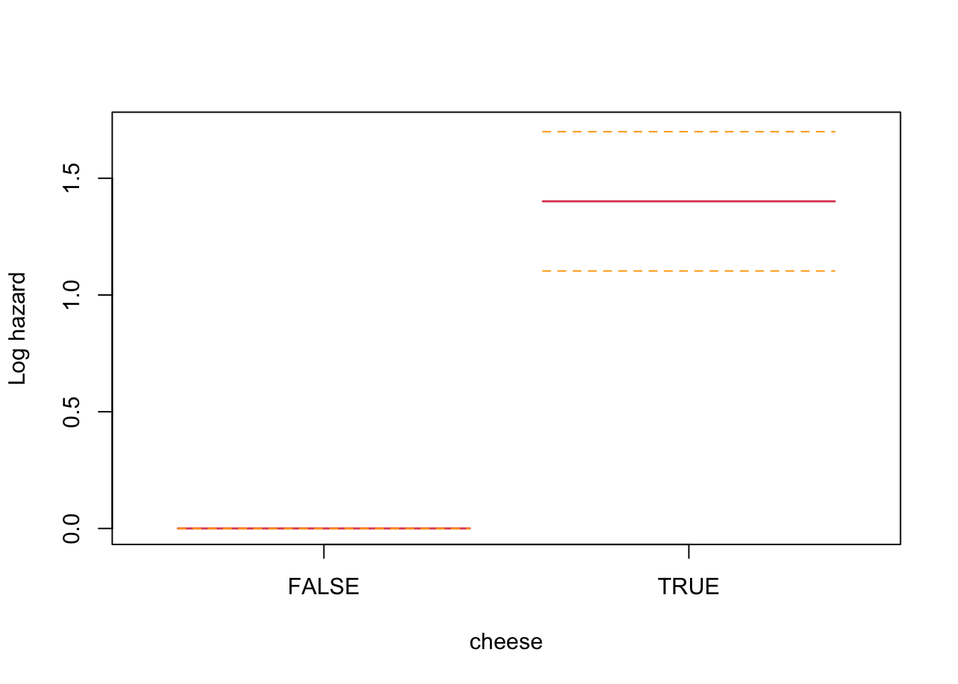
Let’s quickly see how this looks for the cheese trigger to develop some intuition before using it to assess the autoregressive effect of previous night sleeping time.
|
|
This analysis is indicating a log proportional hazard of 1.4012452 for nights with a meal containing cheese (zero for no cheese), which is statistically significant.
Now for the analysis for my autoregressive features of one and two nights previous. I don’t anticipate a linear relationship so I will pass a penalized spline into the model.
|
|
This is an interesting result that differs from the parametric findings. The print out shows a coefficient for each spline’s linear part, and a significance test only for the non-linear part. Sleep time on both the previous night (coef = -0.1021) and two nights previous (coef = -0.1691) have an effect, with two nights previous being slightly larger. Both coefficients are found to be significant and negative, and so inversely proportional. The interpretation is that less time sleeping on previous nights increases the harzard. This runs counter to intuition and the parametric findings. However, R provides a built in plotting function that reveals the relationship very clearly.
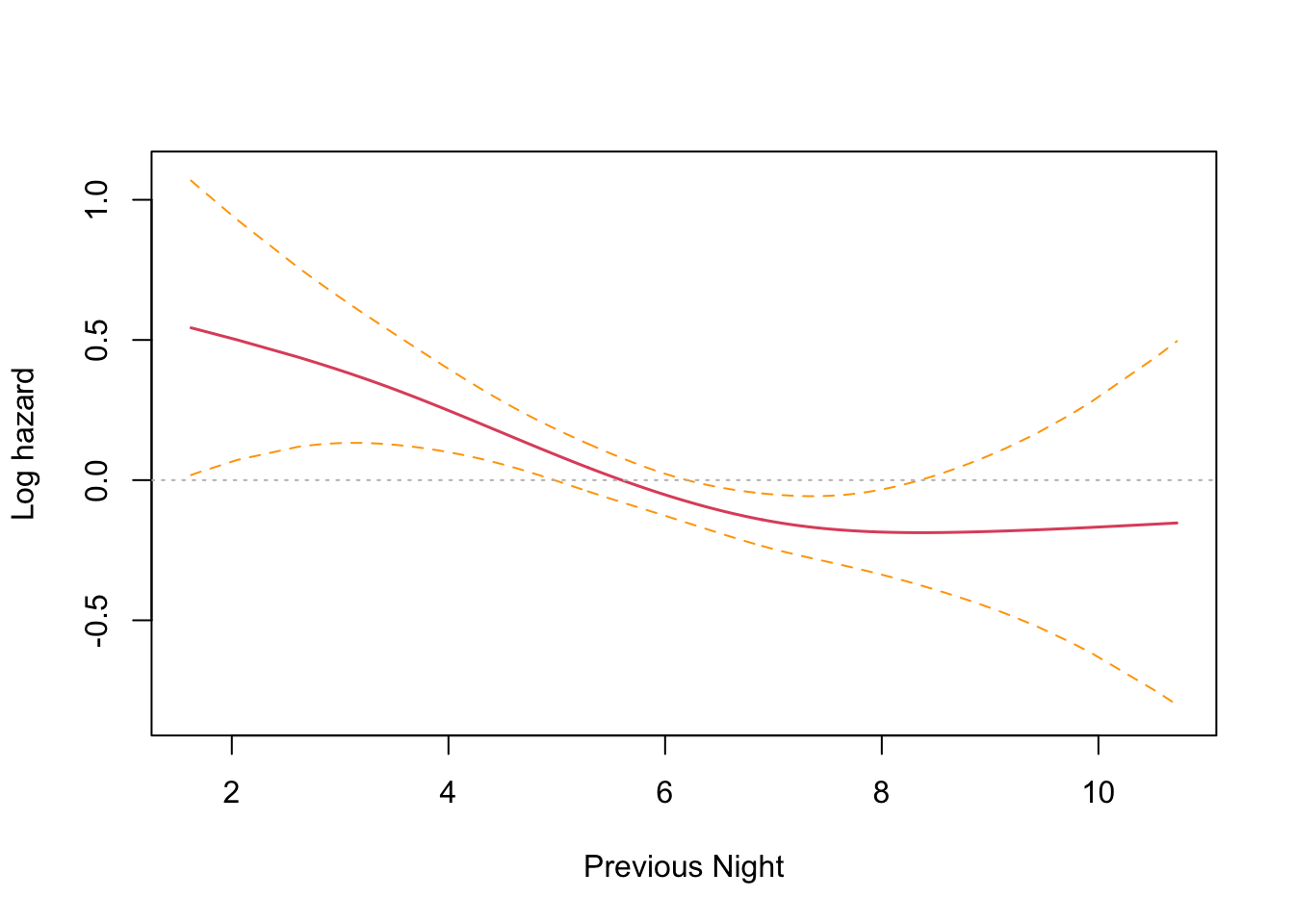
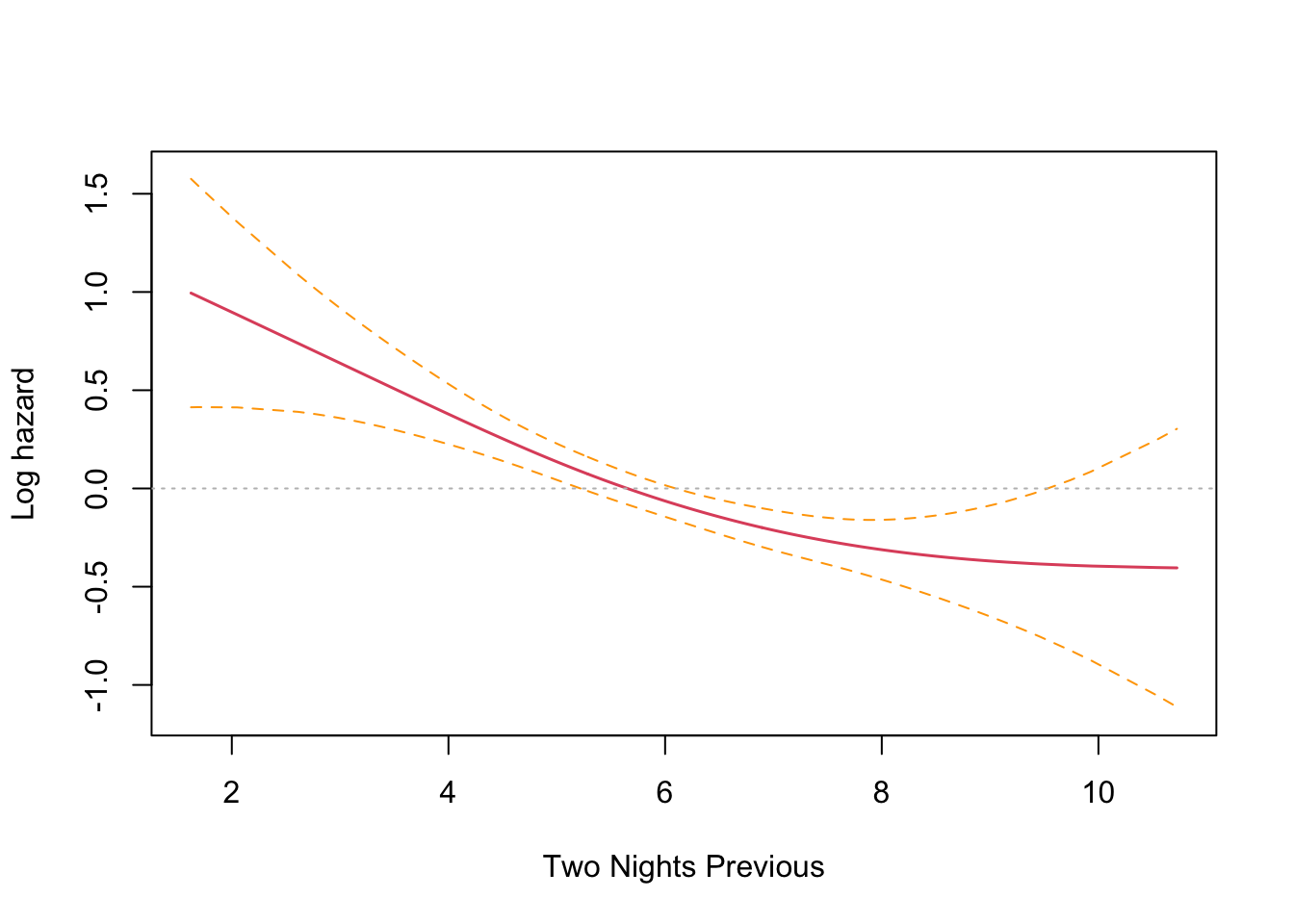
The plots confirm the model results that hazard increases with less sleep on the previous two nights. There is an inflection point somewhere near the median sleep time where the effect is neutral in both cases. The non-intuitive inverse relationship could be a result of not running the other co-factors in the model (something akin to Simpson’s paradox).
Unlike the KM estimator survival curve analysis, it’s more intuitive to run a multivariate proportional hazards regression with many more co-factors. I’ll run the model with the seasonal (month) effect included to see if my hunch is correct.
|
|
Wow! I was absolutely spot on. Controlling for the seasonal effect of just sleeping less in the shorter summer nights, the results are consistent with the findings from last time. Sleep time on the previous night (coef = 0.1051) has a significant effect that is no longer reversed, and two nights previous (coef = -0.0078) no longer has a significant effect.
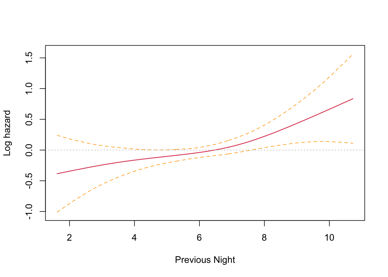
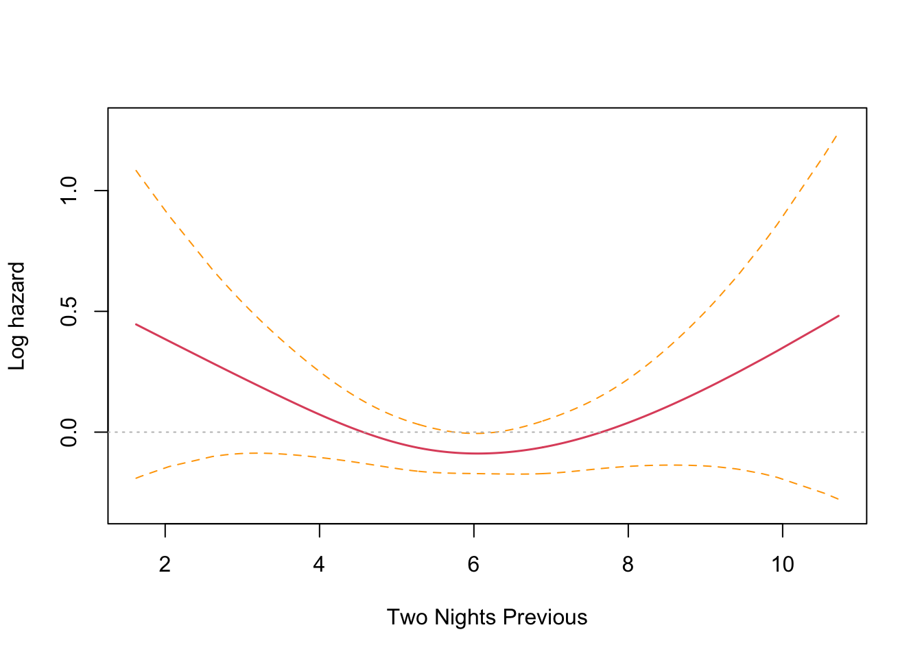
The plots confirm this finding, with previous night hazard appearing to fall monotonically with less sleep, while for two nights previous, the zero reference line is entirely contained inside the confidence interval.
Further work #
It is possible to go further with proportional hazards regression and to select the best model using log-likelihood tests for nested models and AIC for non-nested models. This is familiar territory for linear models and GLMs. I performed this procedure in the previous post on parametric survival analysis. So for the moment, my investigation will end here.
Conclusion #
Running a typical survival analysis on an atypical dataset was an interesting exercise. It did yield a confusing result as I progressed to a more advanced regression analysis with autoregressive continuous variables at first, but this was cleared up by approaching the problem with a critical mindset.
The parametric approach from the previous post yielded a very satisfying analysis because the data was well-fitting to the Weibull distribution, as well as acheiving goodness of fit with a Gamma distribution and normal distribution. However, the non-parametric survival curves yielded by the Kaplan-Meyer estimator actually show you the true, empirical picture of your data set rather than some theoretical distribution. In most cases, this is preferable to work with.
We couldn’t look into some of the aspects of survival analysis that only present themselves in longitudinal studies, such as observations being censored by exiting the study prior to the analysed events. I may return to this topic in a future post.
Overall, it was really great fun to work with a self-generated data set that defines a problem that is pretty core to my personal life. I learned a lot about how to manage my chronic insomnia and that can only be a good thing.
Code Appendix #
|
|
|
|
|
|
|
|
|
|
|
|
|
|
|
|
|
|
|
|
|
|
|
|
|
|
|
|
|
|
|
|
|
|
|
|
|
|
|
|
|
|
|
|
|
|